Randomization distribution and p-values

STAT 120

Bastola

Statistical Hypothesis

  • Null Hypothesis \((H_0):\) Claim that there is no effect or difference.

  • Alternative Hypothesis \((H_a):\) Claim for which we seek evidence.

Always claims about population parameters.

Statistical Significance

Hypothesis testing is similar to how our justice system works (or is suppose to work).

\[\mathrm{H}_{0} : \text{Defendant is innocent vs. } \mathrm{H}_{\mathrm{a}} \text{: Defendant is guilty}\]

Statistical Significance

Assumption: Defendant is innocent \(\left(\mathrm{H}_{0}\right)\)

Verdict:

  • Guilty: evidence (data) “beyond a reasonable doubt” points to guilt (Statistically significant)
  • Not Guilty: evidence (data) not beyond a reasonable doubt, but we don’t know if they are truly innocent \(\left(\mathrm{H}_{0}\right)\)

Randomization Distribution

A randomization distribution is a collection of statistics from samples simulated assuming the null hypothesis is true

  • Also known as a permutation distribution.
  • A randomization distribution is centered at the value of the parameter given in the null hypothesis.

Randomization Distribution for ESP

P-value

The p-value is the chance of obtaining a sample statistic as extreme (or more extreme) than the observed sample statistic, if the null hypothesis is true

  • The p-value can be calculated as the proportion of statistics in a randomization distribution that are as extreme (or more extreme) than the observed sample statistic
  • “extreme” is determined by the alternative hypothesis

StatKey ESP


p-value for ESP

The p-value is the chance of getting at least 3 out of 10 guesses correct, if p = 0.2.

  • P-value is about 0.318.
  • About 31% of the time we would get at least 3 out 10 guesses correct just by chance (no ESP). (interpretation)

Quiz

Which conclusion does this p-value support?

A. Inconclusive, little evidence that supports \(\operatorname{ESP}\left(\mathrm{H}_{\mathrm{a}}\right)\)

B. Borderline, weak evidence for \(\operatorname{ESP}\left(\mathrm{H}_{\mathrm{a}}\right)\)

C. Strong statistically significant evidence for \(\operatorname{ESP}\left(\mathrm{H}_{\mathrm{a}}\right)\)

Click for answer The correct answer is A.

Randomization Distribution: Correlation

Using the randomization distribution below to test

\[\begin{align*} \mathrm{H}_0: \rho=0 \quad \text { vs } \quad \mathrm{H}_{\mathrm{a}}: \rho>0 \end{align*}\]

Match the sample statistics: \(r=0.1\), \(r=0.3\), and \(r=0.5\) with the p-values: \(0.005\), \(0.15\), and \(0.35\). Which sample statistic goes with which p-value?


library(CarletonStats)
FloridaLakes <- read.csv("https://www.lock5stat.com/datasets2e/FloridaLakes.csv")
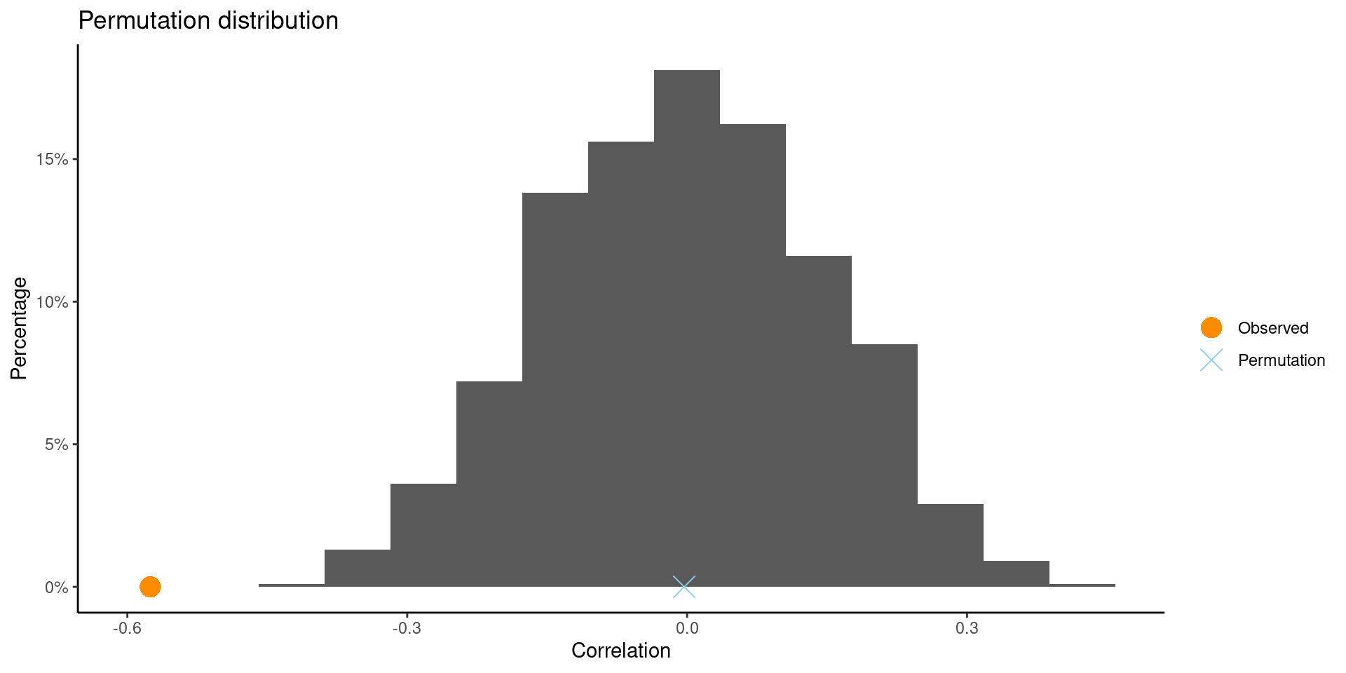
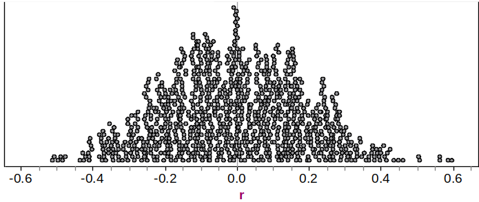
permTestCor(FloridaLakes$pH, FloridaLakes$AvgMercury)

    ** Permutation test **

 Permutation test with alternative: two.sided 
 Observed correlation between FloridaLakes$pH ,  FloridaLakes$AvgMercury : -0.5754 
 Mean of permutation distribution: -0.00314 
 Standard error of permutation distribution: 0.14681 
 P-value:  0.001 

    *-------------*

Alternative Hypothesis

  • A one-sided alternative contains either > or <
  • A two-sided alternative contains \(\neq\)
  • The p-value is the proportion in the tail in the direction specified by \(\mathrm{H}_{\mathrm{a}}\)
  • For a two-sided alternative, the \(\mathrm{p}\)-value is twice the proportion in the smallest tail

p-value and \(H_a\)

\[\begin{align*} \text { Upper-tail } \quad & \mathrm{H}_0: \mu=0 \\ \text { (Right Tail) }\quad & \mathrm{H}_{\mathrm{a}}: \mu>0 \\ \bar{x}& =2 \end{align*}\]

\[\begin{align*} \text { Lower-tail } \quad & \mathrm{H}_0: \mu=0 \\ \text { (Left Tail) } \quad & \mathrm{H}_{\mathrm{a}}: \mu<0 \\ \bar{x}&=-1 \end{align*}\]

\[\begin{align*} \text { Two-tailed } \quad & \mathrm{H}_0: \mu=0 \\ \quad & \mathrm{H}_{\mathrm{a}}: \mu \neq 0 \\ \bar{x}&=2 \end{align*}\]

]


library(CarletonStats)
SleepCaffeine <- read.csv("https://www.lock5stat.com/datasets2e/SleepCaffeine.csv")
permTest(SleepCaffeine$Words, SleepCaffeine$Group)

    ** Permutation test **

 Permutation test with alternative: two.sided 
 Observed statistic
  Caffeine :  12.25      Sleep :  15.25 
 Observed difference: -3 

 Mean of permutation distribution: 0.01755 
 Standard error of permutation distribution: 1.51603 
 P-value:  0.0487 

    *-------------*

Independent vs. Dependent Samples

  • Independent samples: No link between groups’ observations.
  • Dependent samples: Observations are naturally paired.
    • Example: Measurements before and after an intervention.

Hypothesis Testing for Paired Differences: permTestPaired()

  • Focus on the average of within-pair differences, \(\mu_d = \mu_1 - \mu_2\).

  • Hypotheses:

    • \(H_0: \mu_d = 0\) (no effect)
    • \(H_A: \mu_d \neq 0\) (presence of effect)

Coccaine Addiction (Difference in Proportions)

In a randomized experiment, 48 cocaine addicts attempting to quit were randomly assigned to take either desipramine (a new drug) or lithium (an existing drug) to test if desipramine is more effective than lithium at treating cocaine addiction, with relapse as the response variable.

  Relapse No Relapse total
Desipramine 10 14 24
Lithium 18 6 24

Is desipramine more effective than lithium at treating cocaine addiction?

StatKey Coccaine Addiction


  • \(\hat{p}_{D}\): proportion relapsed in Desipramine
\[\begin{aligned} & \mathrm{H}_0: p_{D}=p_{L} \\ & \mathrm{H}_{\mathrm{a}}: p_{D}<p_{L} \end{aligned}\]
  • \(\hat{p}_{L}\): proportion relapsed in Lithium

\[\begin{align*} \hat{p}_{D}=\frac{10}{24}= 0.42 \quad \hat{p}_{L}=\frac{18}{24}= 0.75 \end{align*}\] So the sample statistic is: \[\begin{align*} \hat{p}_{D}-\hat{p}_{L}=0.42-0.75=-0.33 \end{align*}\]

How extreme is -0.33, if \(p_{D}=p_{L}\)?

Randomization steps?

  1. Randomly assign treatments (desipramine/lithium) to 48 participants.

  2. Create many simulated samples, assuming null hypothesis is true.

  3. Shuffle outcomes (relapse/no relapse) without regard to treatment.

  4. Calculate the difference in proportion of relapses for each sample.

  5. Repeat steps c and d multiple times (1000+)

StatKey Coccaine Addiction


p-value ≈ 0.021

StatKey Coccaine Addiction


p-value ≈ 0.021

If proportion relapse for desipramine
is the same as that for lithium,
we would see differences this extreme
about 2.1% of the time

p-value and \(H_0\)

  • If the p-value is small, then a statistic as extreme as that observed would be unlikely if the null hypothesis were true, providing statistically “discernible” evidence against \(\mathrm{H}_0\)

  • The smaller the p-value, the stronger the evidence against the null hypothesis and in favor of the alternative

 Group Activity 1


30:00