[1] 1.644854Hypothesis Tests and Confidence Intervals using Normal Distribution!
STAT 120
How do Malaria parasites impact mosquito behavior?
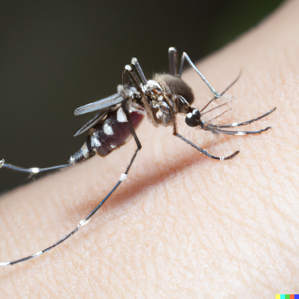
Mosquitoes are tested with two mouse groups: Malaria-infected (experimental) and Healthy (control)
Stages of malaria in mice:
Stage 1: Non-infectious (Days 1-8)Stage 2: Infectious (Days 9-28)Response Variable: Whether the mosquito approaches a human.
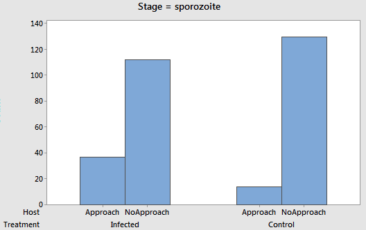
Sample data
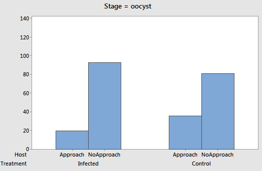
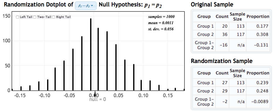
p̂E - p̂C = 20/113 - 36/117 = 0.177 - 0.308 = -0.131
Randomization Distribution
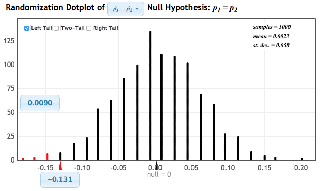
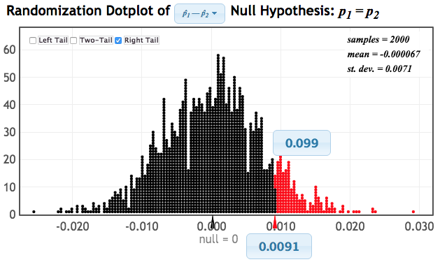
What do you notice?
Which normal distribution?
\[\begin{aligned}
A. \quad & \mathrm{N}(0,-0.131) \\
B. \quad& \mathrm{N}(0,0.056) \\
C. \quad& \mathrm{N}(-0.131,0.056) \\
D. \quad& \mathrm{N}(0.056,0)
\end{aligned}\]
Click for answer
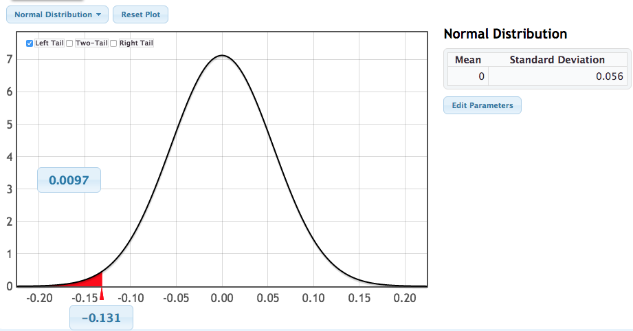
The correct answer is B. (since the distribution is centered at 0 and has standard deviation of 0.056)Statkey: p-value from N(null, SE)
Before and after
p̂E - p̂C =
20/113 - 36/117 =
0.177 - 0.308 = -0.131
p̂E - p̂C =
37/149 - 14/144 =
0.248 - 0.097 = 0.151
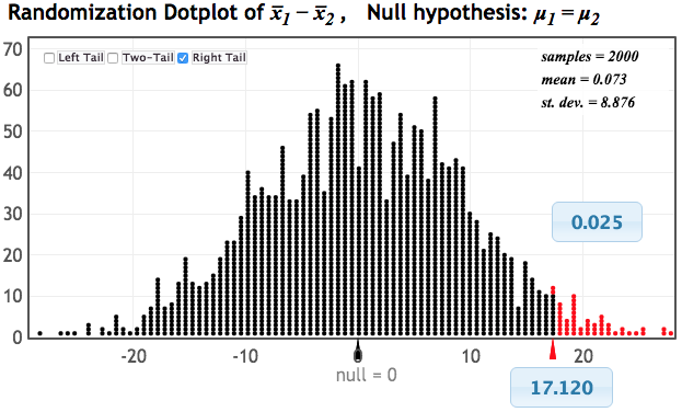
Is the difference significant?
The difference in proportions is 0.151 and the standard error is 0.05. Is this significant?
A. Yes
B. No
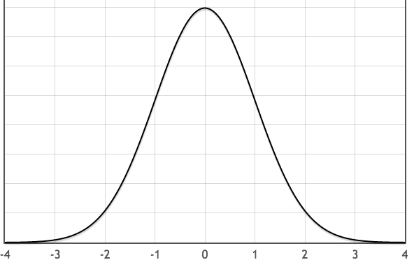
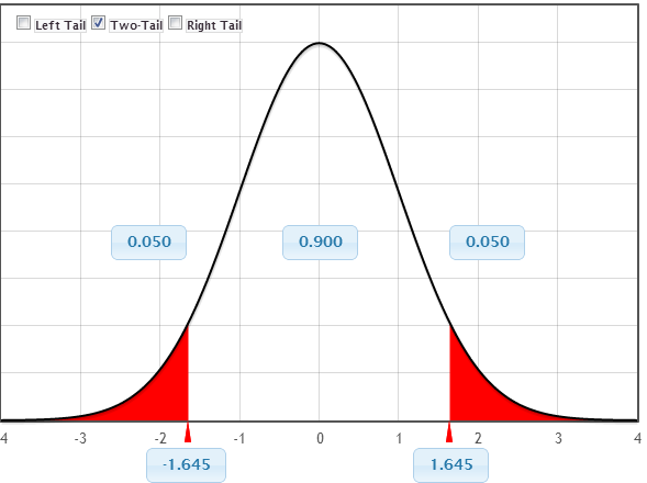
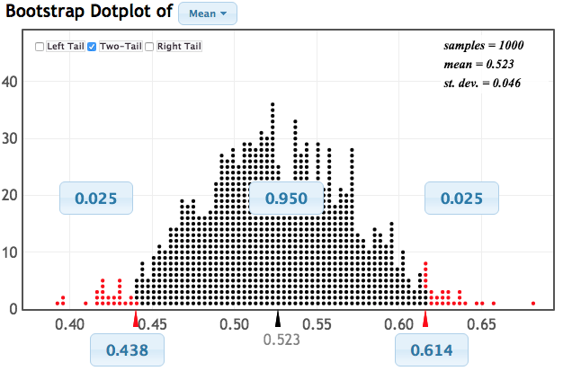
N(0,1) model
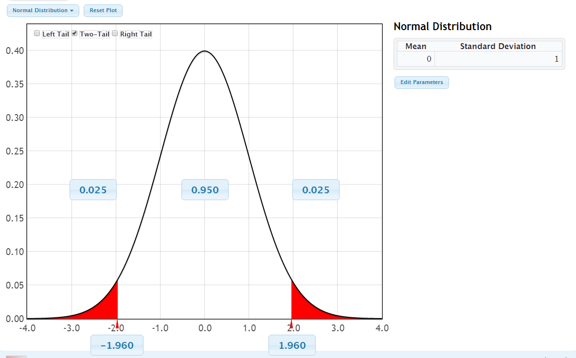
95% of all values fall within 1.96 SE’s of the mean
What if we wanted a 90% CI? What z-score should we use?

Group Activity 1

- Please download the Class-Activity-16 template from moodle and go to class helper web page
30:00