[1] 0Inference for Single Proportions using the Normal Distribution
STAT 120
Bastola
Recap: Why are most resampling distributions bell-shaped?
CLT: when n is big enough, means and proportions behave like a normal distribution.
- Today we will compute SE using formulas derived from probability theory
- The inference methods in ch. 6+ are “classical” methods that could be done just with pen and paper.
The big question: Resampling vs. Classical methods
- Resampling methods are intuitive and don’t require lots of statistical theory/background.
- But in your research fields you will likely only see classical methods used
- In the “olden days”, classical methods were the only thing taught in stats methods classes.
- More advanced methods usually do rely on classical theory due to their complexity.
Quiz
The Central Limit Theorem applies to the distribution of the
- statistic
- parameter
- null value
- data
- standard error
Click for answer
1. (since CLT gives us condition under which the sampling distribution of sample means and proportions follow the normal distribution!)Distribution of sample proportions
The SE for a Sample Proportion
The standard error for \(\hat{p}\) is \[\begin{align*} S E_{\hat{p}}=\sqrt{\frac{p(1-p)}{n}} \end{align*}\]
The larger the sample size (n), the smaller the SE
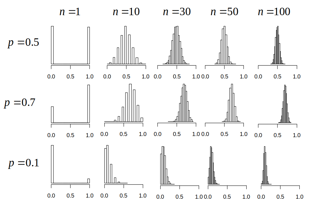
Central Limit Theorem
For a sufficiently large sample size, the distribution of sample statistics for a mean or a proportion is normal
- One sample proportion] The sampling distribution for a sample proportion is approximately normally distributed:
\[\begin{align*} \hat{p} \approx N\left(p, \sqrt{\frac{p(1-p)}{n}}\right) \end{align*}\]
Need n large enough so np ≥ 10 and n(1 – p) ≥ 10
Election polling
President Biden won 52.4% of the popular vote in Minnesota in the 2020 election.
- If we had sampled 100 likely voters just prior to the election, what would be the SE for the sample proportion of voters for Biden?
\[\begin{align*} S E=\sqrt{\frac{0.524 \times 0.476}{100}} \approx 0.05 \end{align*}\]
Margin of Error
For a single proportion, what is the margin of error (ME)?
\[\begin{align*} \hat{p} \pm z^* \times \sqrt{\frac{\hat{p}(1-\hat{p})}{n}} \end{align*}\]
- \(\sqrt{\frac{\hat{p}(1-\hat{p})}{n}}\)
- \(z^* \times \sqrt{\frac{\hat{p}(1-\hat{p})}{n}}\)
- \(2 \times z^* \times \sqrt{\frac{\hat{p}(1-\hat{p})}{n}}\)
Click for answer
The correct answer is 2. (since margin of error is a numerical multiple of SE that is determined by how much confidence we want on the confidence interval)Margin of Error (ME) and Sample Size (n)
\[\begin{align*} M E=z^* \times \sqrt{\frac{\hat{p}(1-\hat{p})}{n}} \end{align*}\]
You can choose your sample size in advance, depending on your desired margin of error!
Given the formula for margin of error, solve for n.
Neither \(p\) nor \(\hat{p}\) is known in advance. To be conservative, use \(p=0.5\). For a \(95 \%\) confidence interval, \(z^* \approx 2\)
\[\begin{align*} n=\left(\frac{z^*}{M E}\right)^2 \hat{p}(1-\hat{p}) \qquad \Longleftrightarrow \qquad n \approx \frac{1}{M E^2} \end{align*}\]
Margin of Error (ME) and \(p\) for fixed \(n\)
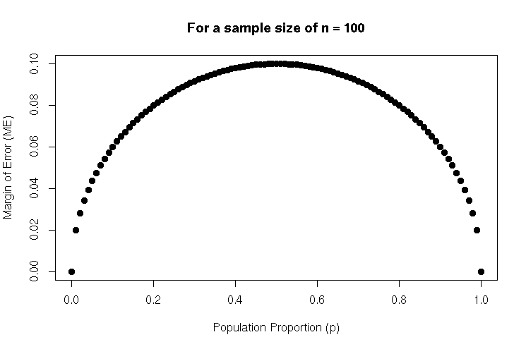
Maximized at p = 0.5
When our sample suggests an even split,
there’s more room for variability,
leading to a larger ME
Margin of Error and n: \(n \approx \frac{1}{M E^2}\)
Suppose we want to estimate a proportion with a margin of error of 0.03 with 95% confidence. How large a sample size do we need?
- About 100
- About 500
- About 1000
- About 5000
Click for answer
The correct answer is 3.Election polling continued..
What should n be to get a margin of error of 3%?
\[\begin{gathered} 0.03=2 \times \text { SE } \\ 0.015=S E=\sqrt{\frac{0.482 \times 0.518}{n}} \\ n=\frac{0.524 \times 0.476}{0.015^2} \approx 1109 \end{gathered}\]Test for a Single Proportion: Standardized Test Stat and P-value
\[\begin{align*} \mathrm{H}_0: & \quad p=p_0\\ \mathrm{H}_A: & \quad p\neq p_0 \end{align*}\]
\[\begin{align*} z&=\frac{\hat{p} -p_0}{\sqrt{\frac{p_0\left(1-p_0\right)}{n}}} \end{align*}\]
If \(np_0 ≥ 10\) and \(n(1 – p_0) ≥ 10\), then the p-value can be computed as the area in the tail(s) of a standard normal beyond z.
Global Warming
A survey on 2,251 randomly selected individuals conducted in October 2010 found that 1328 answered “Yes” to the question. Do a majority of Americans believe in global warming?
\[\begin{aligned} & H_0: p=0.50 \\ & H_A: p>0.50 \end{aligned}\]\[p=\text { proportion of all Americans who believe in global warming }\]
“Is there solid evidence of global warming?”
Source: “Wide Partisan Divide Over Global Warming”, Pew Research Center, 10/27/10.s
Global warming continued: Is there solid evidence of global warming?
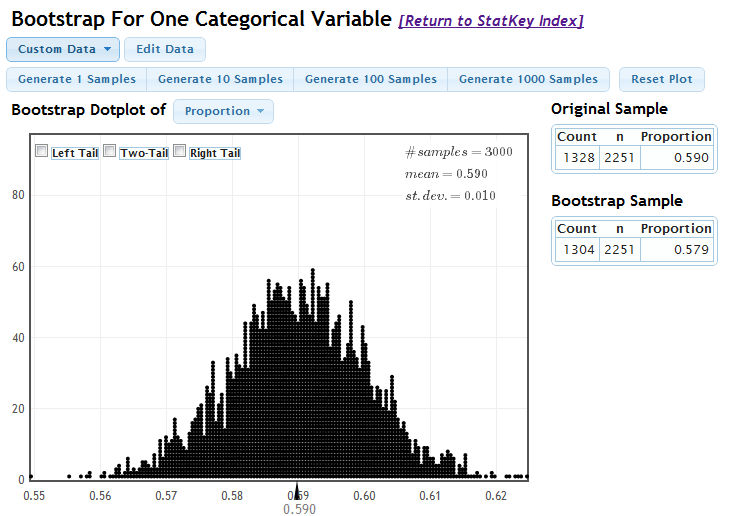
Sample proportion: \[\begin{align*} \hat{p}=\frac{1328}{2251}=0.590 \end{align*}\]
Standardized test stat: \[\begin{align*} z=\frac{0.590-0.50}{\sqrt{\frac{0.50(0.50)}{2251}}}=\frac{0.09}{0.0105}=8.54 \end{align*}\]
P-value:
C.I. for p: \(\hat{p} \pm z^* \sqrt{\frac{\hat{p}(1-\hat{p})}{n}}\)
\[\begin{align*} 0.59 \pm& 1.96 \sqrt{\frac{0.59 \times(1-0.59)}{2251}} \\ 0.59 \pm& 1.96 \times 0.0104 = (0.570,0.610) \end{align*}\]
Correct Interpretation
P-value: proportion above z=8.54 on a N(0,1) curve. Yes, there is statistically discernible evidence that the percentage of Americans that believe in global warming is greater than 50% (z=8.51, \(p \approx 0\)).
We are 95% confident that between 57% and 61% of Americans believe in global warming.
Statkey: Does this agree with the bootstrap CI?
We are 95% sure that
the true percentage of all Americans
that believe there is solid evidence
of global warming is between
57.0% and 61.0%.
Summary
Standard error for a sample proportion: Central Limit Theorem for a proportion: If counts for each category are at least 10 (meaning \(n p \geq 10\) and \(n(1-p) \geq 10)\), then
- For a \(\mathrm{CI}\), use \(p\)-hat in place of \(p\)
- For a Hypothesis Test, use \(p_0\) in place of \(p\) when calculating the standardized statistic
Group Activity 1

- Please download the Class-Activity-17 template from moodle and go to class helper web page
30:00