Inference for one mean
STAT 120
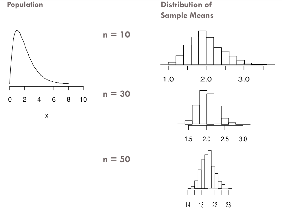
CLT for mean
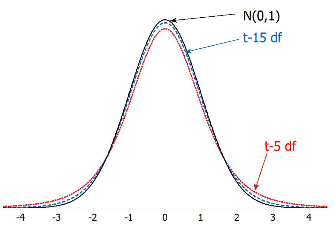
T-distribution
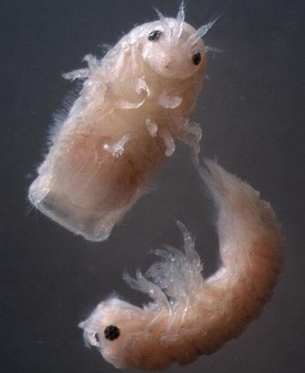
Gribbles
Gribbles are small marine worms that bore through wood, and the enzyme they secrete may allow us to turn inedible wood and plant waste into biofuel
A sample of 50 gribbles finds an average length of \(3.1 \mathrm{~mm}\) with a standard deviation of \(0.72 \mathrm{~mm}\).
Give a \(90 \%\) confidence interval for the average length of gribbles.
Gribbles
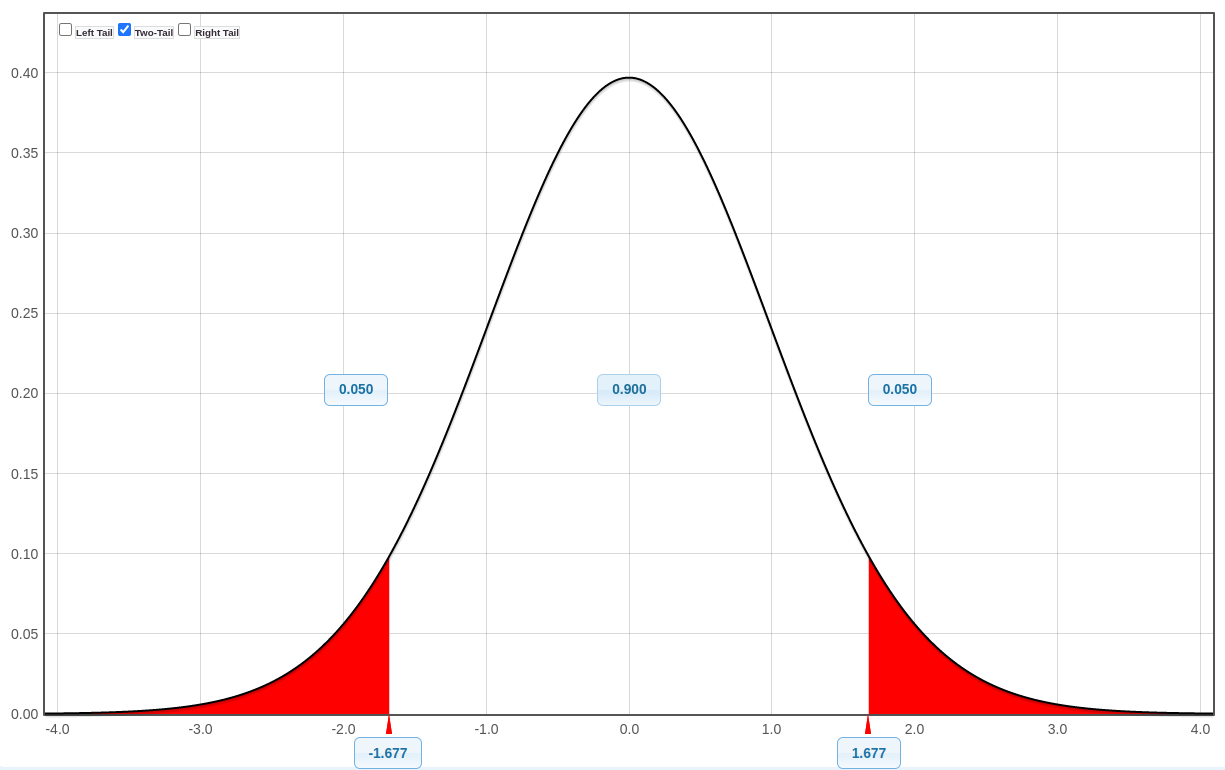
A sample of 50 gribbles finds an average length of \(3.1 \mathrm{~mm}\) with a standard deviation of \(0.72 \mathrm{~mm}\). For a \(90 \%\) confidence interval for the average length of gribbles, what is \(t^*\) ?
a). 1.645 b). 1.677 c). 1.960 d). 1.690
Click for answer
\(d f=n-1=49 \text { and } t^*=1.677\) Gribbles
A sample of 50 gribbles finds an average length of \(3.1 \mathrm{~mm}\) with a standard deviation of \(0.72 \mathrm{~mm}\). For a \(90 \%\) confidence interval for the average length of gribbles, what is the standard error?
a). 0.171 b). 0.720 c). 1.960 d). 0.102
Click for answer
\(\frac{s}{\sqrt{n}}=\frac{0.72}{\sqrt{50}}=0.102\) Gribbles
A sample of 50 gribbles finds an average length of \(3.1 \mathrm{~mm}\) with a standard deviation of \(0.72 \mathrm{~mm}\). For a \(90 \%\) confidence interval for the average length of gribbles, what is the margin of error?
a). 0.171 b). 0.720 c). 1.960 d). 0.102
Click for answer
\(t^* \cdot \frac{s}{\sqrt{n}}=1.677 \cdot \frac{0.72}{\sqrt{50}}=0.171\) Gribbles
\(\begin{gathered}\text { statistic } \pm t^* \cdot S E \\ \bar{x} \pm t^* \cdot \frac{s}{\sqrt{n}} \\ 3.1 \pm 1.677 \cdot \frac{0.72}{\sqrt{50}} \\ 3.1 \pm 0.17 \\ (2.93,3.27)\end{gathered}\)
We are \(90 \%\) confident that the average length of gribbles is between 2.93 and \(3.27 \mathrm{~mm}\).