Inference for two means
STAT 120
The SE for means
The standard error for \(\bar{x}\) is \[S E_{\bar{x}}=\frac{\sigma}{\sqrt{n}}\] where \(\sigma\) is the population SD of your response
The standard error for \(\bar{x}_{1}-\bar{x}_{2}\) is \[S E_{\bar{x}_{1}-\bar{x}_{2}}=\sqrt{\frac{\sigma_{1}^{2}}{n_{1}}+\frac{\sigma_{2}^{2}}{n_{2}}}\]
But we usually do not know \(\sigma\) !
- Estimate \(\sigma\) with the sample SD \(s\)
Central Limit Theorem for means: One sample
The sampling distribution for a sample mean, \(\bar{x}\), is approximately \(N\left(\mu, S E_{\bar{x}}\right)\)
When is this approximately “good”?
if \(X \sim N(\mu, \sigma)\) then \(\bar{X} \sim N(\mu, \sigma / \sqrt{n})\)
if \(X \nsim N(\mu, \sigma)\) then \(\bar{X} \sim N(\mu, \sigma / \sqrt{n})\) if \(n \geqslant 30\)
Central Limit Theorem for means: Two independent samples:
The sampling distribution for a difference of two independent sample means is approximately \(N\left(\mu_{1}-\mu_{2}, S E_{\bar{x}_{1}-\bar{x}_{2}}\right)\)
When is this approximately “good”?
- need both \(n_{1}\) and \(n_{2}\) samples sizes big enough for the one-sample condition
Academic Performance Index (API)
Academic Performance Index (API) is a number reflecting a school’s performance on a statewide standardized test
- simple random sample of \(n=200\) schools
- variable
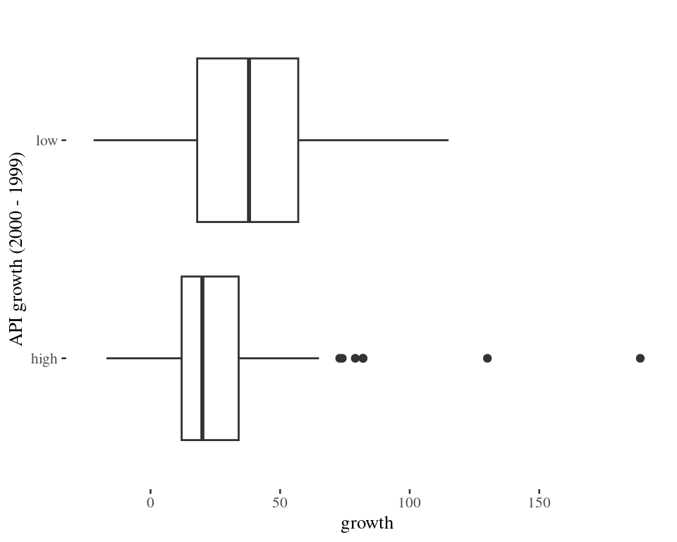
growthmeasures the growth in API from 1999 to 2000 (API 2000 - API 1999).
Academic Performance Index (API)
API
Hypothesis Test
Can we use t-inference methods to compare mean growths?
Both samples sizes (98 and 102) can be deemed large
No severe skewness (but two extreme outliers)
Estimated Standard Error : \(SE_{\bar{x}_h - \bar{x}_l} = \sqrt{\dfrac{28.75380^2}{102} + \dfrac{29.95048^2}{98}} = 4.1544\)
Test statistics: \(t = \dfrac{(25.24510 - 38.82653) - 0}{4.154404} = -3.2692\)
The observed mean difference is 3.3 SEs below the hypothesized mean difference of 0
Two-sample t-test
    Welch Two Sample t-test

data:  growth by wealth
t = -3.2692, df = 196.71, p-value = 0.001273
alternative hypothesis: true difference in means between group high and group low is not equal to 0
95 percent confidence interval:
 -21.774321  -5.388544
sample estimates:
mean in group high  mean in group low
          25.24510           38.82653
The p-value is 0.001273. If there is no difference between mean growth in the two populations, then there is just a 0.13% chance of seeing a sample mean difference that is 3.27 standard errors or more away from 0.
Outliers
           cds stype            name                 sname snum
1 5.471911e+13     E Lincoln Element    Lincoln Elementary 5873
2 1.975342e+13     E Washington Elem Washington Elementary 2543
                    dname dnum       cname cnum flag pcttest api00 api99 target
1 Exeter Union Elementary  226      Tulare   53   NA      98   693   504     15
2   Redondo Beach Unified  585 Los Angeles   18   NA     100   745   615      9
  growth sch.wide comp.imp both awards meals ell yr.rnd mobility acs.k3 acs.46
1    189      Yes      Yes  Yes    Yes    50  18   <NA>        9     18     NA
2    130      Yes      Yes  Yes    Yes    41  20   <NA>       16     19     30
  acs.core pct.resp not.hsg hsg some.col col.grad grad.sch avg.ed full emer
1       NA       93      28  23       27       14        8   2.51   91    9
2       NA       81      11  26       32       16       16   2.99  100    3
  enroll api.stu    pw  fpc wealth
1    196     177 30.97 6194   high
2    391     313 30.97 6194   high
t.test with outliers removed
    Welch Two Sample t-test

data:  growth by wealth
t = -4.395, df = 174.97, p-value = 1.916e-05
alternative hypothesis: true difference in means between group high and group low is not equal to 0
95 percent confidence interval:
 -23.571116  -8.961945
sample estimates:
mean in group high  mean in group low
          22.56000           38.82653
How does removing outliers influence t-test stat and p-value?
Confidence Interval
95% Confidence Interval from the output:
- Without Outliers: (-23.57, -8.96)
- With Outliers: (-21.77, -5.39)
Removing Outliers:
- the difference in means shifted further away from 0
- CI shifted further from a difference of 0
- decrease the SE of our sample difference
Interpretation: We are 95% confident that the mean API growth between 1999 and 2000 for all low wealth schools is anywhere from 8.96 points to 23.57 points higher than the mean API growth for all high wealth schools in California.
Paired Data
Data are paired if the data being compared consists of paired data values. Common paired data examples:
- Two measurements on each case
- natural pairs (twins, spouses, etc)
Use paired data to reduce natural variation in the response when comparing the two groups/treatments
- comparing group 1 and 2 responses among similar individuals
- reduces the effects of confounding variables
- reduces the SE for the mean difference!
Analyzing paired data
Look at the difference between responses for each unit (pair) \[d_{i} = x_{1,i} - x_{2,i}\]
Analyze the mean of these differences rather than the average difference between two groups \[\textrm{sample mean difference: } \bar{d}\] \[\textrm{sample SD of difference: } s_d\] \[\textrm{population mean difference: } \mu_d\]
Use one sample inference methods for these differences
Tuition example
How much higher is non-resident tuition, on average, compared to resident tuition? Use the Tuition2006.csv lab manual data
- the variable
Diffcomputes the differenceRes-NonRes
tuition <- read.csv("http://math.carleton.edu/Stats215/RLabManual/Tuition2006.csv")
head(tuition)
##   X        Institution  Res NonRes  Diff
## 1 1 Univ of Akron (OH) 4200   8800 -4600
## 2 2  Athens State (AL) 1900   3600 -1700
## 3 3    Ball State (IN) 3400   8600 -5200
## 4 4  Bloomsburg U (PA) 3200   7000 -3800
## 5 5     UC Irvine (CA) 3400  12700 -9300
## 6 6 Central State (OH) 2600   5700 -3100
Tuition example: Histogram and QQ-plot

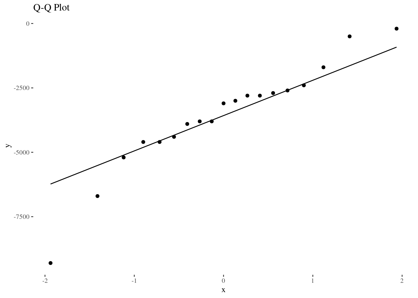
Tuition example: t-test
# alternate method
t.test(tuition$Res, tuition$NonRes, paired = TRUE)
##
##  Paired t-test
##
## data:  tuition$Res and tuition$NonRes
## t = -7.5349, df = 18, p-value = 5.69e-07
## alternative hypothesis: true mean difference is not equal to 0
## 95 percent confidence interval:
##  -4583.580 -2584.841
## sample estimates:
## mean difference
##       -3584.211
We are 95% confident that the mean tuition for non-residents is $2585 to $4584 higher than mean tuition for residents
Group Activity 1

- Please download the Class-Activity-21 template from moodle and go to class helper web page
30:00