Inference for multiple proportions: One Categorical Variable
STAT 120
Tests for One Categorical Variable
Goodness-of-fit test
- Test a claim about the distribution of one categorical variable
- E.g. are 6 M&M colors equally likely?
- E.g. is Biden’s approval rating 50%?
Tests for One Categorical Variable
Seen single proportion tests before - Example : Test if the proportion of Reese’s Pieces that are orange is different from 1/3.
\[\begin{aligned} H_0 : p = 1/3\\ H_a : p \neq 1/3 \end{aligned}\]What if we want to test proportions for several categories at once?
- Example: Are the three colors (orange, yellow, brown) of Reese’s Pieces equally likely?
\(H_0\) specifies a proportion, \(p_i\) , for each category.
Rock-Paper-Scissors
| ROCK | PAPER | SCISSORS | TOTAL |
|---|---|---|---|
| 36 | 12 | 37 | 85 |
How would we test whether all of these categories are equally likely?
Conduct a hypothesis test
- State Hypothesis
- Calculate a test statistic, based on your sample data
- Create a distribution of this statistic, as it would be observed if the null hypothesis were true
- Measure how extreme your test statistic is, as compared to the distribution generated under null
Test Statistic
Why can’t we use the familiar formula to get the test statistic?
\[\frac{\text { sample statistic - null value }}{\text { SE }}\]
- More than one sample statistic
- More than one null value
We need something a bit more complicated …
Observed Counts
The observed counts are the actual counts observed in the study
| ROCK | PAPER | SCISSORS | TOTAL |
|---|---|---|---|
| 36 | 12 | 37 | 85 |
- The expected counts are the expected counts if the null hypothesis were true
- For each cell, the expected count is the sample size \(n\) times the null proportion, \(p_o\)
| ROCK | PAPER | SCISSORS | TOTAL | |
|---|---|---|---|---|
| Observed | 36 | 12 | 37 | 85 |
| Expected | 28.33 | 28.33 | 28.33 | 85 |
Chi-Square Statistic
- A test statistic is one number, computed from the data, which we can use to assess the null hypothesis
- The chi-square statistic is a test statistic for categorical variables:
Rock-Paper-Scissors
| ROCK | PAPER | SCISSORS | TOTAL | |
|---|---|---|---|---|
| Observed | 36 | 12 | 37 | 85 |
| Expected | 28.33 | 28.33 | 28.33 | 85 |
What next?
We have a test statistic. What else do we need to perform the hypothesis test? - A distribution of the test statistic assuming \(H_0\) is true
How do we get this? Two options:
- Simulation
- Theoretical Distribution
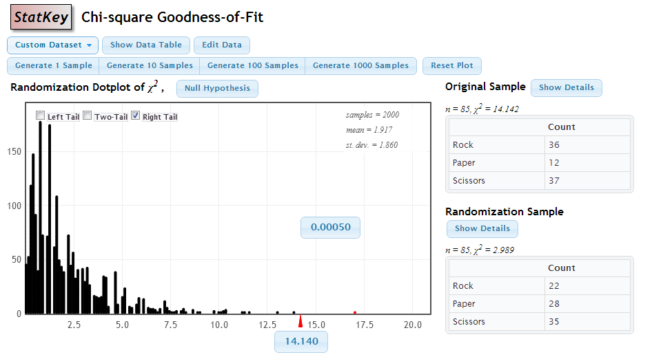
Simulation
Take 3 scraps of paper and label them Rock, Paper, Scissors. Fold or crumple them so they are indistinguishable. Choose one at random and record the result.
Repeat a number of times to match the original sample size and get a table of observed counts.
Calculate the \(\chi^{2}\)-statistic.
Repeat this many times to get a randomization distribution of many \(\chi^{2}\)-statistics.
How extreme is the actual test statistic in this randomization distribution?
Statkey: Chi-Square Distribution
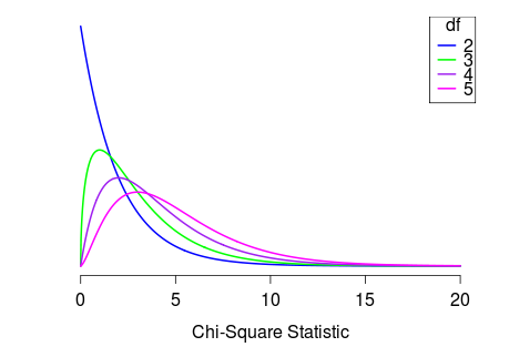
Chi-Square Distribution
If each of the expected counts are at least 5, AND if the null hypothesis is true, then the \(\chi^2\) statistic follows a \(\chi^2\) distribution, with degrees of freedom equal to
\[df = \text{number of categories} -1\]
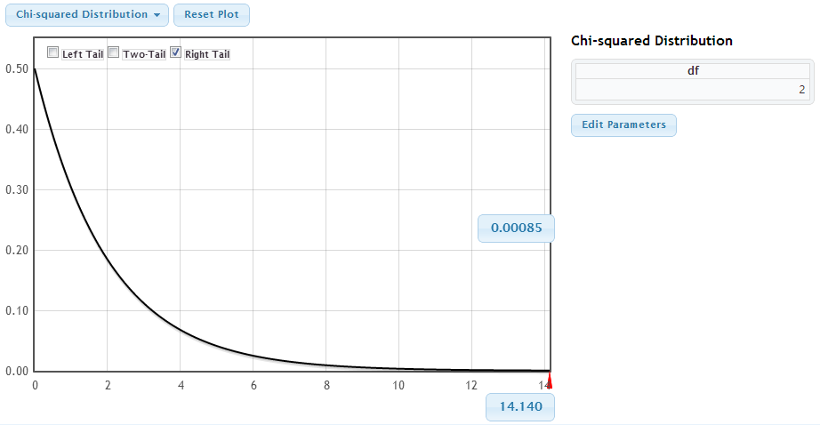
Rock-Paper-Scissors:
df = 3 - 1 = 2 # degrees of freedom Chi-Square Distribution
Statkey: p-value using Chi-square distribution
Goodness of Fit
A \(\chi^2\) test for goodness of fit test determines whether the distribution of a categorical variable is the same as some null hypothesized distribution
The null hypothesized proportions for each category do not have to be the same
Chi-Square Test for Goodness of Fit
State null hypothesized proportions for each category, pi. Alternative is that at least one of the proportions is different than specified in the null.
Calculate the expected counts for each cell as \(n\cdot p_i\). Make sure they are all greater than 5 to proceed.
Calculate the \(\chi^2\) statistic: \(\chi^2 = \sum{\frac{(observed - expected)^2}{expected}}\)
Compute the p-value as the area in the tail above the \(\chi^2\) statistic, for a \(\chi^2\) distribution with \(df = (\text{number of categories - 1})\).
Interpret the p-value in context and conclude.
Group Activity 1

- Please download the Class-Activity-22 template from moodle and go to class helper web page
30:00