Inference for multiple proportions: Two Categorical Variables

STAT 120

Bastola

Tests for Categorical Variable(s)

Chi-square test for association

  • Determine if a relationship between two categorical variables is statistically significant
  • E.g. Does M&M color distribution depend on type (chocolate vs. peanut)?

Chi-square test for association hypothesis

Hypotheses look like:

\[H_0: \textrm{two categorical variables are not associated}\] \[H_A: \textrm{two categorical variables are associated}\]

E.g. Does M&M color distribution depend on type (chocolate vs. peanut)?

\[H_0: \text{there is no association between M&M color and type}\] \[H_A: \text{there is an association between M&M color and type}\]

Expected Counts and p-value

The expected counts for each combination in a two-way table

\[\textrm{expected count} = \dfrac{\textrm{row total} \times \textrm{column total}}{n}\]

\[\chi^2 = \sum_{\textrm{all cells}}\dfrac{(\textrm{Observed} - \textrm{Expected})^2}{\textrm{Expected}}\]

  • Large chi-square test stat values support the alternative hypothesis so: \(p-value = P(\chi^2 \geq \text{observed } \chi^2)\)

  • always a right-tailed value

Chi-Square test for association: P-VALUE

randomization/permutation: simulate new data consistent with \(H_0\) and recompute the \(\chi^2\) test stat

  • Association: permute the values of one variable column to break the link that could exist in the data between both variables

Chi-square distribution (probability model):

  • Association: use \((r-1)(c-1)\) where \(r=\) number of rows and \(c=\) number of columns
  • need \(n\) large enough so expected counts are at least 5

Example: Does political comfort level depend on religion?

\(H_0:\) There is no association between religion and comfort level

  • implies: the distribution of comfort level is the same for all three religion types

\(H_A:\) There is an association between religion and comfort level

  • implies: the distribution of comfort level is the different for at least one religion type.

Association example

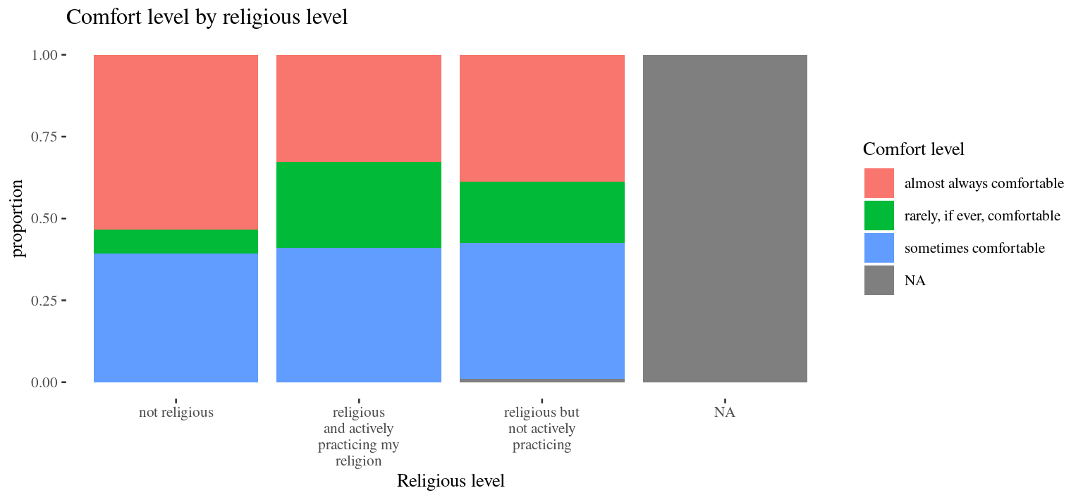
survey <- read.csv("https://raw.githubusercontent.com/deepbas/statdatasets/main/Survey.csv")
survey %>% dplyr::select(Question.8, Question.9) %>% head()
                             Question.8                Question.9
1                         not religious almost always comfortable
2                         not religious     sometimes comfortable
3                         not religious almost always comfortable
4 religious but not actively practicing almost always comfortable
5                         not religious     sometimes comfortable
6                         not religious almost always comfortable
Table 1: A two way table of religious preference and political comfortness
almost always comfortable rarely, if ever, comfortable sometimes comfortable
not religious 110 15 81
religious and actively practicing my religion 20 16 25
religious but not actively practicing 41 20 44

Association example

Association Example

EDA for two categorical variables

  • drop missing values, rename column names
  • change/shorten comfort level names
  • reorder the levels

Observed distribution of political comfort level given religiousness

Table 2: A two way table of religious preference and political comfortness (cleaned-up factors)
almost always sometimes rarely
not religious 103 76 15
religious not active 39 41 19
religious active 18 24 15

Association example

counts <- table(survey$religiousness, survey$comfortness)
counts
##                       
##                        almost always sometimes rarely
##   not religious                  103        76     15
##   religious not active            39        41     19
##   religious active                18        24     15
prop.table(counts,1)  
##                       
##                        almost always  sometimes     rarely
##   not religious           0.53092784 0.39175258 0.07731959
##   religious not active    0.39393939 0.41414141 0.19191919
##   religious active        0.31578947 0.42105263 0.26315789

There is a much higher rate of “almost always” comfortable for the not religious respondents (53.1%) than those that are religious (not active: 39.4%; active: 31.6%).

Association example

Association example

Expected counts assuming no association (null)?

  • expected number of respondents who are “not religious” and “almost always comfortable”?
  • is not 1/9 of all respondents!

Association example

  • There are 194 “not religious” respondents (row total)

  • The overall rate (ignoring religion) of “almost always comfortable” is \(\dfrac{160}{350}\), or about 45.7%.

  • If religion isn’t related to comfort level, the expected number is about \[\textrm{expected count} = \dfrac{\textrm{row total} \times \textrm{column total}}{n} = 194 \times \dfrac{160}{350} = 88.686\]

Association example

Chi-square contribution for “not religious” and “almost always comfortable” cell?

  • The contribution to the chi-square test stat from this category is 2.31.

\[\dfrac{(103 - 88.686)^2}{88.686} = 2.31\]

Association example: chisq.test

ComfortReligion <- chisq.test(survey$religiousness, survey$comfortness)
ComfortReligion

    Pearson's Chi-squared test

data:  survey$religiousness and survey$comfortness
X-squared = 19.33, df = 4, p-value = 0.0006768
  • The test stat value is 19.33.
  • There are 3 categories for each variable, so the degrees of freedom will be \(df = (3-1)(3-1) = 4\).

Association example

  • Interpret: If there is no association between comfort level and religiousness, then we would see a chi-square test stat of 19.33, or one even larger, only about 0.07% of the time.

  • Conclusion: We have strong evidence that there is an association between political comfort level and religiousness ( \(\chi^2 = 19.33\), df = 4, p-value = 0.0007).

Association example: Check Assumptions!

Are the expected counts above 5?

ComfortReligion <- chisq.test(survey$religiousness, survey$comfortness)
ComfortReligion$expected
                      survey$comfortness
survey$religiousness   almost always sometimes rarely
  not religious             88.68571  78.15429  27.16
  religious not active      45.25714  39.88286  13.86
  religious active          26.05714  22.96286   7.98

Association example

  • If we get a red warning when running chisq.test, it usually means the sample size conditions aren’t met to use the chi-square model.

  • Instead run a randomization test with simulate.p.value = TRUE

chisq.test(survey$religiousness, survey$comfortness, 
           simulate.p.value = TRUE)

    Pearson's Chi-squared test with simulated p-value (based on 2000
    replicates)

data:  survey$religiousness and survey$comfortness
X-squared = 19.33, df = NA, p-value = 0.0009995

Association example

Describe the association!

  • which groups have the most different comfort levels?

Association example

95% CI for the difference in the true proportions of “rarely comfortable” people in the not religious and actively religious groups. \[p = \textrm{proportion rarely comfortable}\]

  • 95% CI for \(p_{not.relig} - p_{active}\)
table(survey$religiousness)

       not religious religious not active     religious active 
                 194                   99                   57 

\[n_{not.relig} = 194 \ \ \ \ \ \ n_{active} = 57\]

Association example

knitr::kable(counts)
almost always sometimes rarely
not religious 103 76 15
religious not active 39 41 19
religious active 18 24 15
knitr::kable(round(prop.table(counts,1),3))
almost always sometimes rarely
not religious 0.531 0.392 0.077
religious not active 0.394 0.414 0.192
religious active 0.316 0.421 0.263

\[\hat{p}_{not.rel} = \dfrac{15}{194} = 0.0773196\] \[\hat{p}_{active} = \dfrac{15}{57} = 0.2631579\]

Association example

95% CI for \(p_{not.relig} - p_{active}\)

\[\begin{align*} 0.0773196 - 0.2631579 \pm & 1.96 \sqrt{\dfrac{0.0773196(1-0.0773196)}{194} + \dfrac{0.2631579(1-0.2631579)}{57}} \\ -0.1858383 \pm & 1.96 (0.061397) \\ (-0.3061765, & -0.0655001) \end{align*}\]

I am 95% confident that the percentage of all non-religious students who are rarely comfortable is between 6.6 to 30.6 percentage points lower than the actively religious students.

 Group Activity 1


30:00