Comparing Two or more Means
STAT 120
Frisbee Example
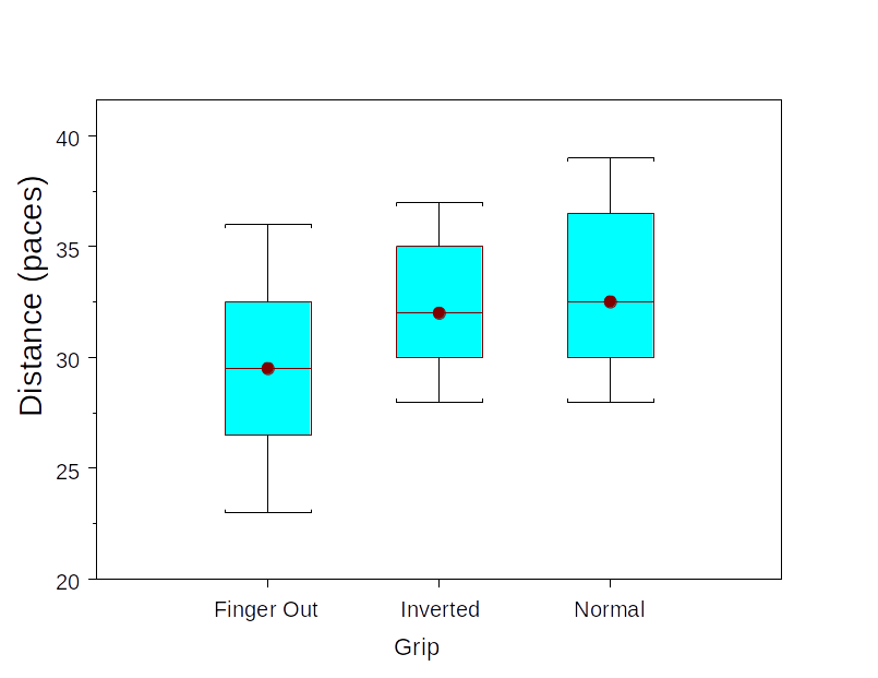
| Finger-out | Inverted | Normal | |
|---|---|---|---|
| n | 8 | 8 | 8 |
| Mean | 29.5 | 32.375 | 33.125 |
| SD | 4.175 | 3.159 | 3.944 |
Question: Is this evidence that grip affects mean distance thrown? \[\begin{align*} H_{0}:& \quad \mu_{1}=\mu_{2}=\mu_{3}\\ H_{a}:& \quad \text{At least one } \mu_{1}, \mu_{2}, \mu_{3} \text{ is not the same} \end{align*}\]
:::
Why Analyze Variability to Test for a Difference in Means?
The group means in Datasets \(A\) and \(B\) are the same, but the boxes show different spread.
Datasets \(A\) and \(C\) have the same spread for the boxes, but different group means.
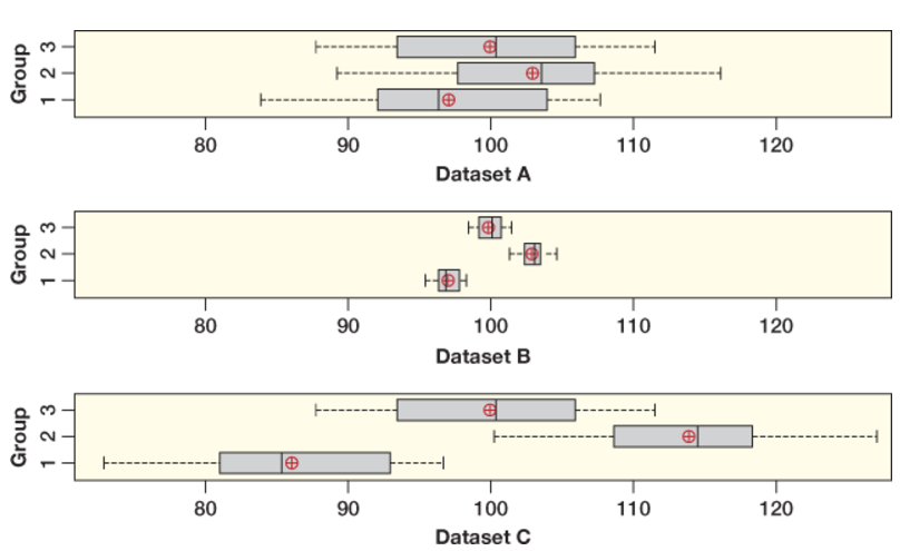
Which of these graphs appear to give strong visual evidence for a difference in the group means?
Why Analyze Variability to Test for a Difference in Means?
Dataset A = weakest evidence for a difference in means.
Datasets B and C = strong evidence for a difference in means.
Why Analyze Variability to Test for a Difference in Means?
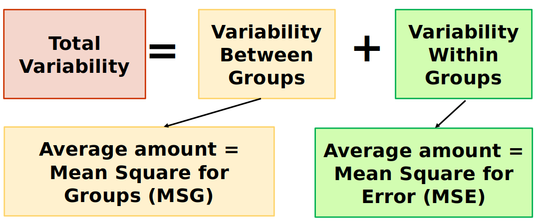
Conclusion: An assessment of the difference in means between several groups depends on two kinds of variability:
- How different the means are between each groups
- The amount of variability within each groups
Analysis of Variance
Analysis of Variance (ANOVA) compares the variability between groups to the variability within groups
CarletonStats R package
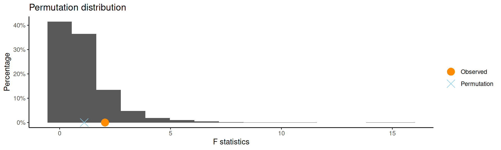
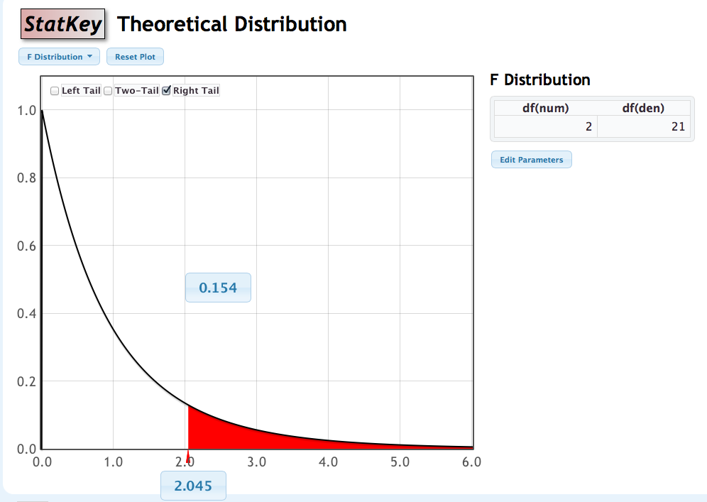
F-distribution
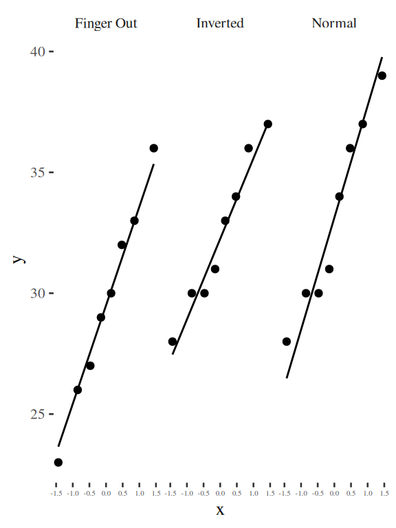
Check assumptions: normality
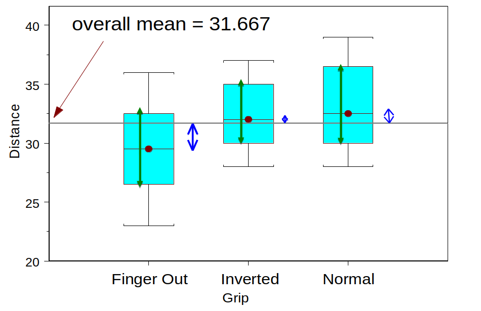
Picturing the variation
Green: Variation within groups
Blue: Variation between groups
Group Activity 1

- Please download the Class-Activity-24 template from moodle and go to class helper web page
30:00