Describing Categorical Variables

STAT 120

Bastola

Descriptive Statistics

In order to make sense of data, we need ways to summarize and visualize it
Summarizing and visualizing variables and relationships between two variables is often known as descriptive statistics, also known as exploratory data analysis (EDA)
The type of summary statistics and visualization methods depend on the type of variable(s) being analyzed (categorical or quantitative)

One Categorical Variable

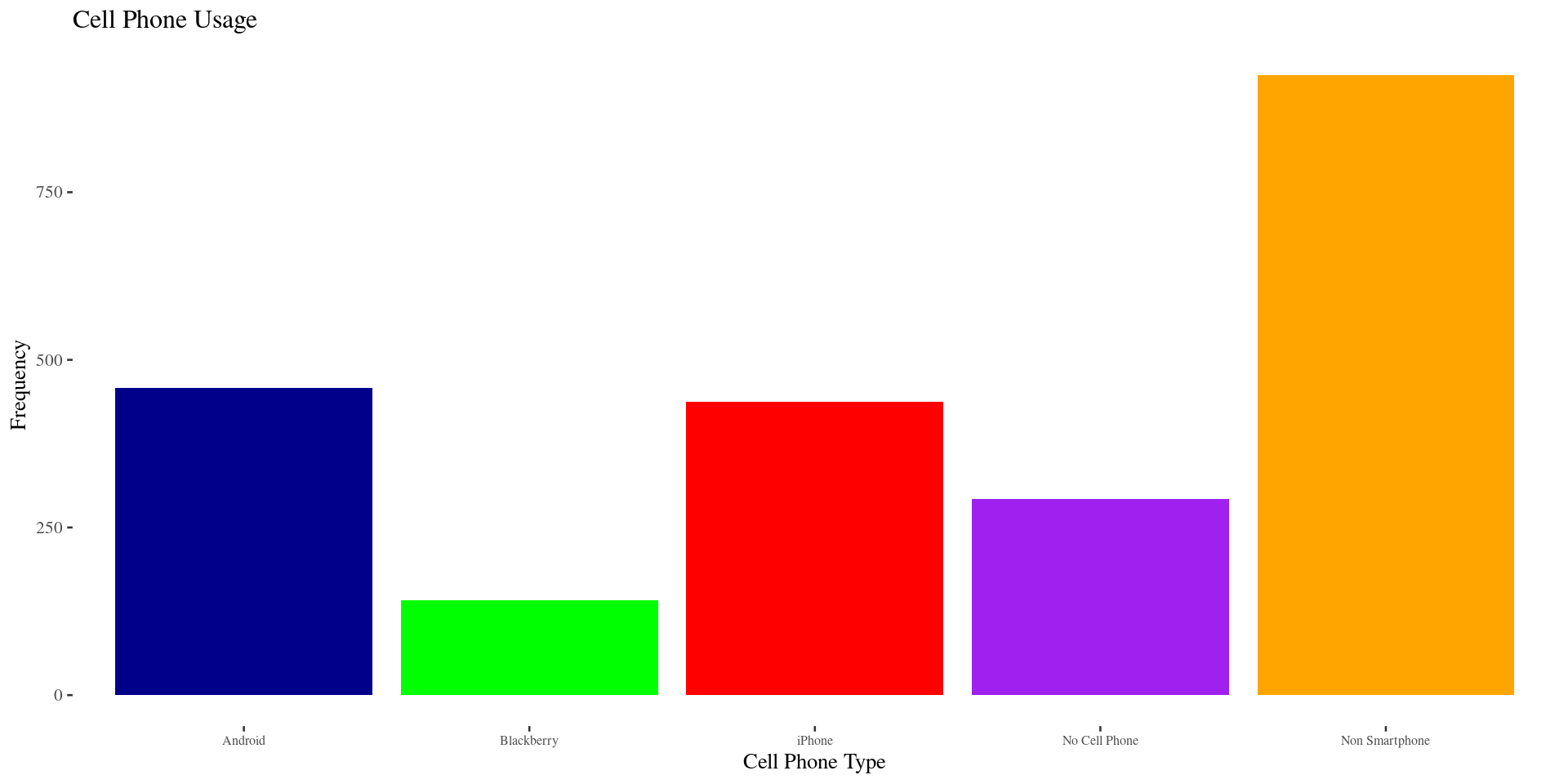
A random sample of US adults in 2012 were surveyed regarding the type of cell phone owned

Android? iPhone? Blackberry? Non-smartphone? No cell phone?

Frequency Table

A frequency table shows the number of cases or counts that fall in each category:

Subset of Raw Data	Device Type
Case 1	Android
Case 2	none
Case 3	none
Case 4	iPhone
Case 5	Non Smartphone
Case 6	iPhone
Case 7	Blackberry
Case 8	Non Smartphone
Case 9	Android
Case 10	Android
…	(for 2253 cases …)

Cell Phone Type	Frequency
Android	458
iPhone	437
Blackberry	141
Non Smartphone	924
No Cell Phone	293
Total	2253

Proportion

The proportion in a category is found by \[\text{proportion} = \frac{\text{number in category}}{\text{total sample size}}\]

Percentages/proportions (relative frequencies)

\(p\) = proportion for a population (parameter)
\(\hat{p}\) = proportion for a sample (statistic) (“p-hat”)

What proportion of adults sampled do not own a cell phone?

Cell Phone Type	Frequency	Proportion
Android	458	0.203
iPhone	437	0.194
Blackberry	141	0.063
Non Smartphone	924	0.41
No Cell Phone	293	0.13
Total	2253	1.000

Proportions and percentages can be used interchangeably

Distribution of a variable

The “distribution of variable Y” describes the count or percent of observations that fall into each category of “variable Y”

E.g. In the 2020 election, 51.3% of voters voted for Biden, 46.8% for Trump and 1.8% for third-party candidates

Bar Chart/Plot/Graph

In a barplot, the height of the bar corresponds to the number of cases falling in each category

Two Categorical Variables

Look at the relationship between two categorical variables - Relationship status - Gender

	Female	Male	Total
In a Relationship	32	10	42
It’s Complicated	12	7	19
Single	63	45	108
Total	107	62	169

We add a second dimension to a frequency table to account for the second categorical variable

Relationship status and Gender

Proportion of students in a relationship that are female?

prop.relation.female <- 32/42
round(prop.relation.female,2)

[1] 0.76

Proportion of students in a relationship that are male?

prop.relation.male <- 10/42
round(prop.relation.male,2)

[1] 0.24

Relationship status and Gender

Proportion of males that are in a relationship?

prop.male <- 10/62
round(prop.male,2)

[1] 0.16

Proportion of females that are in a relationship?

prop.female <- 32/107
round(prop.female,2)

[1] 0.3

Statkey for Data Visualization: https://www.lock5stat.com/StatKey/index.html

Difference in proportions

A difference in proportions is a difference in proportions for one categorical variable calculated for different levels of the other categorical variable

Example: Difference in proportions of male and female that are in a relationship:

\[\begin{align} \text{prop}_{\text{Females}} &- \text{prop}_{\text{Males}}\\ &= \hat{p}_F - \hat{p}_M \\ &= \frac{32}{107} - \frac{10}{62} \\ &= 0.14 \end{align}\]

# R-code
prop.female <- 32/107
prop.male <- 10/62
prop.diff <- prop.female - prop.male
round(prop.diff,2)

[1] 0.14

Case Study: `Flowers v. Mississippi`

2019 Supreme Court case: Has Mississippi prosecutor Doug Evans deliberately use “peremptory challenges” to strike black jurors from jury pools?

American Public Media journalist collected trial data from this district from 1992 to 2017 Link

The data set APM_DougEvansCases.csv contains data on 1517 jurors for cases which listed Doug Evans as the first prosecutor.

Only looking at jurors with race listed as Black or White.
These jurors are eligible for Evans to strike.

Look at the data

jurors <- read.csv("https://raw.githubusercontent.com/deepbas/statdatasets/main/APM_DougEvansCases.csv")
head(jurors)

  trial__id  race        struck_state defendant_race      same_race
1         4 Black Not struck by State          White different race
2         4 Black     Struck by State          White different race
3         4 White Not struck by State          White      same race
4         4 White Not struck by State          White      same race
5         4 Black     Struck by State          White different race
6         4 White Not struck by State          White      same race
                      struck_by
1 Juror chosen to serve on jury
2           Struck by the state
3 Juror chosen to serve on jury
4         Struck by the defense
5           Struck by the state
6 Juror chosen to serve on jury

Look at the data

dim(jurors) # dimension of dataset

[1] 1517    6

Look at the first three rows of the data set

jurors[c(1,2,3),]   #jurors[rows, columns]

  trial__id  race        struck_state defendant_race      same_race
1         4 Black Not struck by State          White different race
2         4 Black     Struck by State          White different race
3         4 White Not struck by State          White      same race
                      struck_by
1 Juror chosen to serve on jury
2           Struck by the state
3 Juror chosen to serve on jury

Look at the data

jurors$struck_state[1:20] # first 20 entries in the `struck_state` variable

 [1] "Not struck by State" "Struck by State"     "Not struck by State"
 [4] "Not struck by State" "Struck by State"     "Not struck by State"
 [7] "Struck by State"     "Not struck by State" "Not struck by State"
[10] "Not struck by State" "Not struck by State" "Not struck by State"
[13] "Struck by State"     "Not struck by State" "Not struck by State"
[16] "Not struck by State" "Struck by State"     "Not struck by State"
[19] "Struck by State"     "Not struck by State"

Numeric summaries: counts and proportions

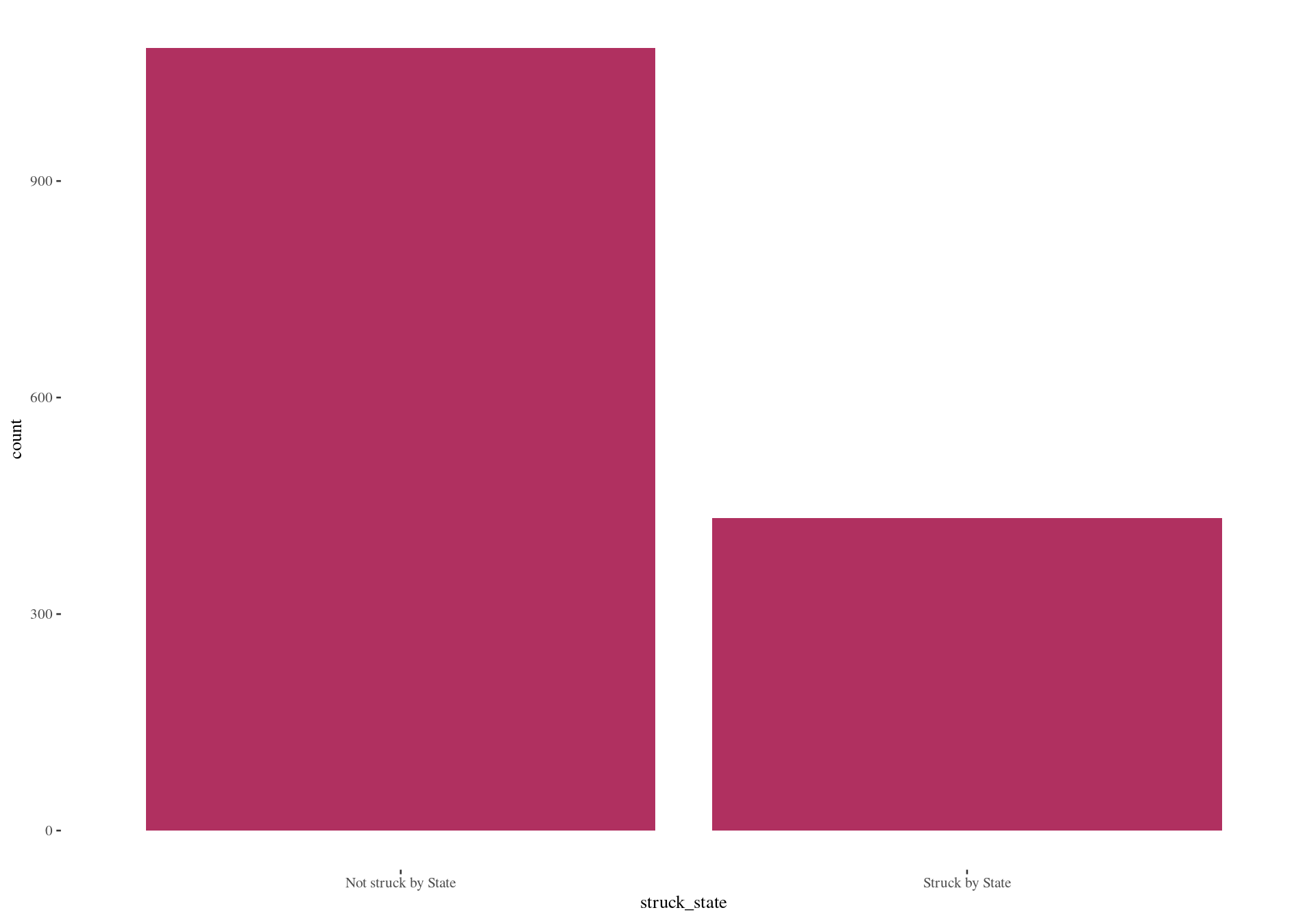
table() gives counts of whether the state struck a juror:

counts <- table(jurors$struck_state)
counts


Not struck by State     Struck by State 
               1084                 433

prop.table() turns these counts into proportions:

prop.table(counts)


Not struck by State     Struck by State 
          0.7145682           0.2854318

What proportion of eligible jurors were struck by the state from the jury pool?

Graphical summary: bar plot using ggplot2

library(ggplot2)  # load the library
ggplot(jurors, aes(x=struck_state)) +
  geom_bar(fill="maroon")

Associations between two categorical variables

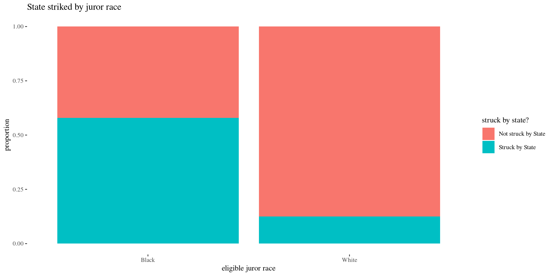
How does state struck status vary by juror race? (How are race and state strikes associated?)

Numerically:

summarize counts in a contingency/two-way table
conditional proportions: “The conditional distribution of Y given variable X” describes how Y is distributed within each category of X (group by X).

Graphically:

stacked bar graph of conditional proportions

Two-way (contingency) table

First 6 entries of race and struck_state variable is

jurors[(1:6), (2:3)]

   race        struck_state
1 Black Not struck by State
2 Black     Struck by State
3 White Not struck by State
4 White Not struck by State
5 Black     Struck by State
6 White Not struck by State

table gives two-way tables when two variables are included.

mytable <- table(jurors$race, jurors$struck_state)
mytable

       
        Not struck by State Struck by State
  Black                 225             310
  White                 859             123

Conditional proportions

prop.table gives conditional proportions grouped by the row variable when margin=1

prop.table(mytable, margin = 1)

       
        Not struck by State Struck by State
  Black           0.4205607       0.5794393
  White           0.8747454       0.1252546

Of all eligible black jurors, about 57.9% were struck by the state.

What proportion of eligible white jurors were struck by the state? Is there evidence of an association between juror race and state strikes?

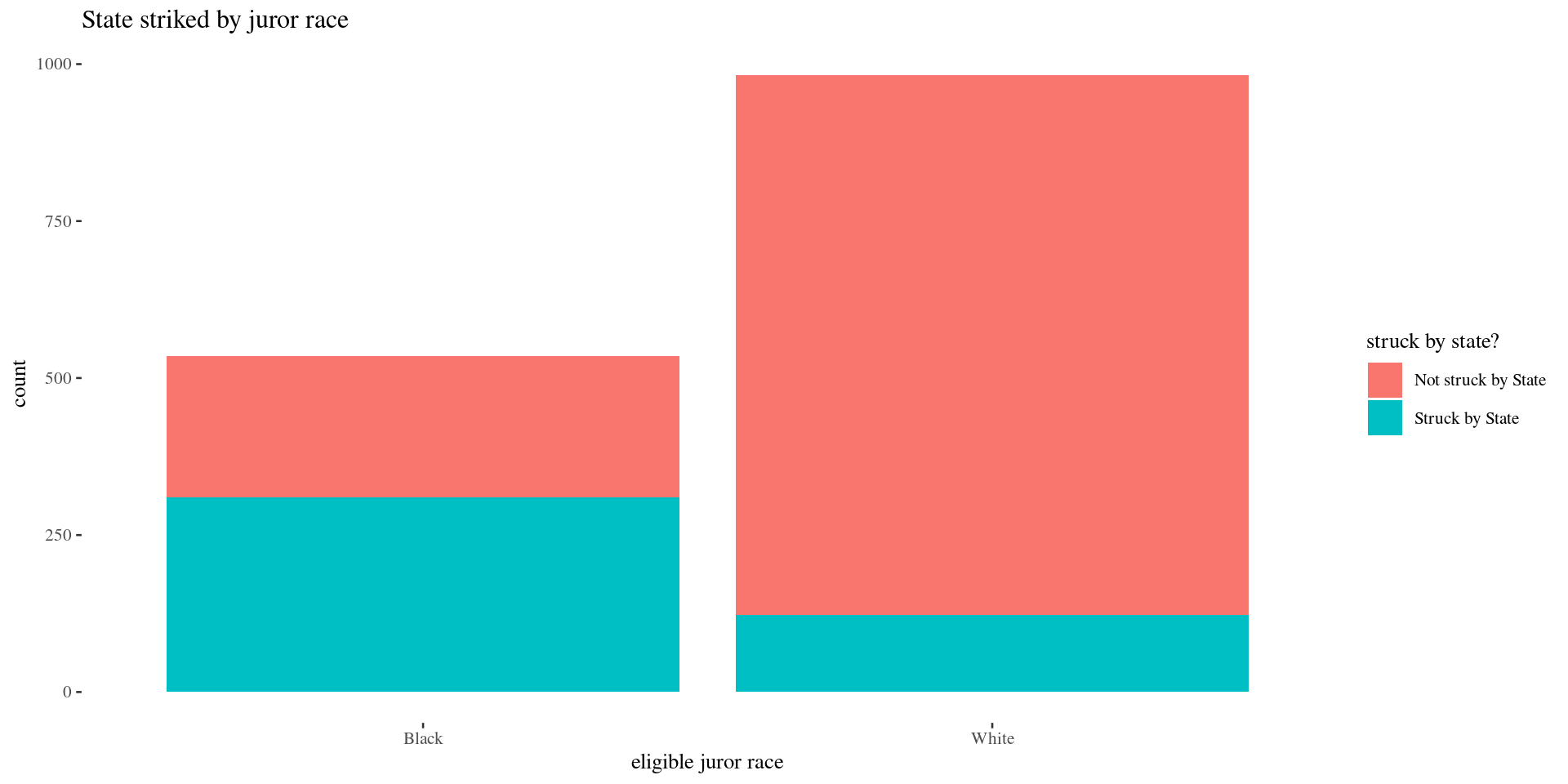
Stacked bar graph

ggplot(jurors, aes(x = race, fill = struck_state)) + 
  geom_bar(position = "fill") + 
  labs(title = "State striked by juror race", 
       y = "proportion", 
       x = "eligible juror race", 
       fill = "struck by state?")

Stacked bar graph (counts)

ggplot(jurors, aes(x = race, fill = struck_state)) + 
  geom_bar(stat="count") + 
  labs(title = "State striked by juror race", 
       y = "count", 
       x = "eligible juror race", 
       fill = "struck by state?")

Please download the Class-Activity-4 template from moodle and go to class helper web page

20:00

Describing Categorical Variables

Descriptive Statistics

One Categorical Variable

Frequency Table

Proportion

What proportion of adults sampled do not own a cell phone?

Distribution of a variable

Bar Chart/Plot/Graph

Two Categorical Variables

Relationship status and Gender

Relationship status and Gender

Difference in proportions

Case Study: Flowers v. Mississippi

Look at the data

Look at the data

Look at the data

Numeric summaries: counts and proportions

Graphical summary: bar plot using ggplot2

Associations between two categorical variables

Two-way (contingency) table

Conditional proportions

Stacked bar graph

Stacked bar graph (counts)

Group Activity 1

Case Study: `Flowers v. Mississippi`