Two Quantitative Variables: Association

STAT 120

Bastola

Describing associations between two quantitative variables

Data: each case \(i\) has two measurements

\(x_i\) is explanatory variable
\(y_i\) is response variable

A scatterplot is the plot of \((x_i, y_i)\)

form? linear or non-linear
direction? positive, negative, no association
strength? amount of variation in \(y\) around a “trend”

Example: Associations in Car dataset

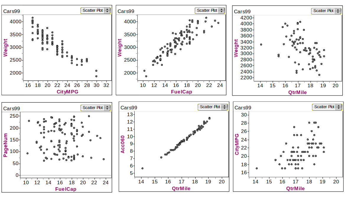
Various Associations of quantitative variables in Cars data

Direction

positive association: as \(x\) increases, \(y\) increases

age of the husband and age of the wife
height and diameter of a tree

negative association: as \(x\) increases, \(y\) decreases

number of cigarettes smoked per day and lung capacity
depth of tire tread and number of miles driven on the tires

Correlation Coefficients

Correlation coefficient: denoted \(r\) (sample) or \(\rho\) (population)

Strength of linear association
- \(r\approx \pm 1:\) strong
- \(r\approx 0:\) weak
Direction of linear association
- \(r > 0:\) positive
- \(r < 0:\) negative

Correlation can be heavily affected by outliers. Plot your data!

R-code:

# order of x and y doesn't matter!
cor(data$x, data$y)

Car Correlations

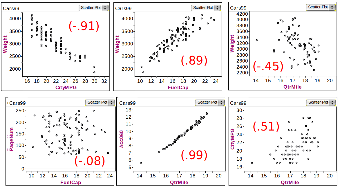
Correlations of various variables in Cars data

Linear Regression

Goal: To find a straight line that best fits the data in a scatterplot

The estimated regression line is \(\hat{y} = a + bx\)

x is the explanatory variable
\(\hat{y}\) is the predicted response variable.

Slope: increase in predicted \(y\) for every unit increase in \(x\) \[ b = \frac{\text{change }\hat{y}}{\text{change } x} \]

Intercept: predicted \(y\) value when \(x = 0\) \[ \hat{y} = a + b(0) = a \]

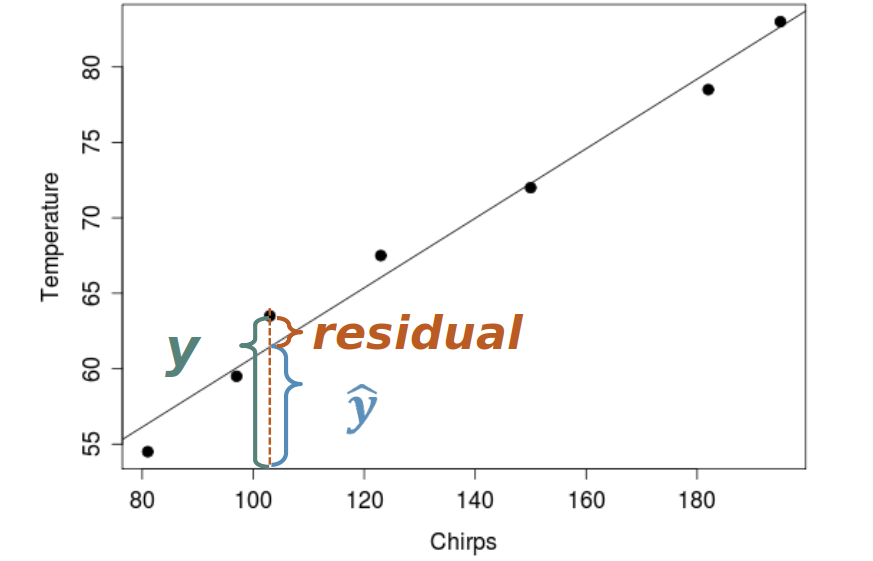
Residuals

Geometrically, residual is the vertical distance from each point to the line

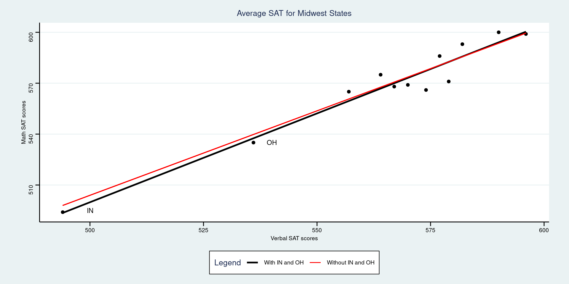
Presence of Outliers

Outliers can be very influential on the regression line. Remove the points and see if the regression line changes significantly

Regression line of Blood Alcohol Content (BAC) data

Regression of BAC on number of beers

bac.lm <- lm(BAC ~ Beers, data=bac) # fit linear model
summary(bac.lm)  # print summary of the model


Call:
lm(formula = BAC ~ Beers, data = bac)

Residuals:
      Min        1Q    Median        3Q       Max 
-0.027118 -0.017350  0.001773  0.008623  0.041027 

Coefficients:
             Estimate Std. Error t value Pr(>|t|)    
(Intercept) -0.012701   0.012638  -1.005    0.332    
Beers        0.017964   0.002402   7.480 2.97e-06 ***
---
Signif. codes:  0 '***' 0.001 '**' 0.01 '*' 0.05 '.' 0.1 ' ' 1

Residual standard error: 0.02044 on 14 degrees of freedom
Multiple R-squared:  0.7998,    Adjusted R-squared:  0.7855 
F-statistic: 55.94 on 1 and 14 DF,  p-value: 2.969e-06

Regression line of Blood Alcohol Content (BAC) data

Slope, \(b= 0.0180\):

Estimate column and Beers row

Intercept, \(a = -0.0127\):

Estimate column and Intercept row

Regressing BAC on number of beers

\[ \widehat{BAC} = -0.0127 + 0.0180(Beers) \]

Slope Interpretation?

Each additional beer consumed is associated with a \(0.0180\) unit increase in BAC

y-intercept Interpretation?

Predicted BAC with 0 beers consumed

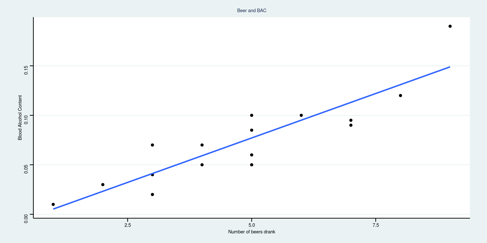
Regressing BAC on number of beers

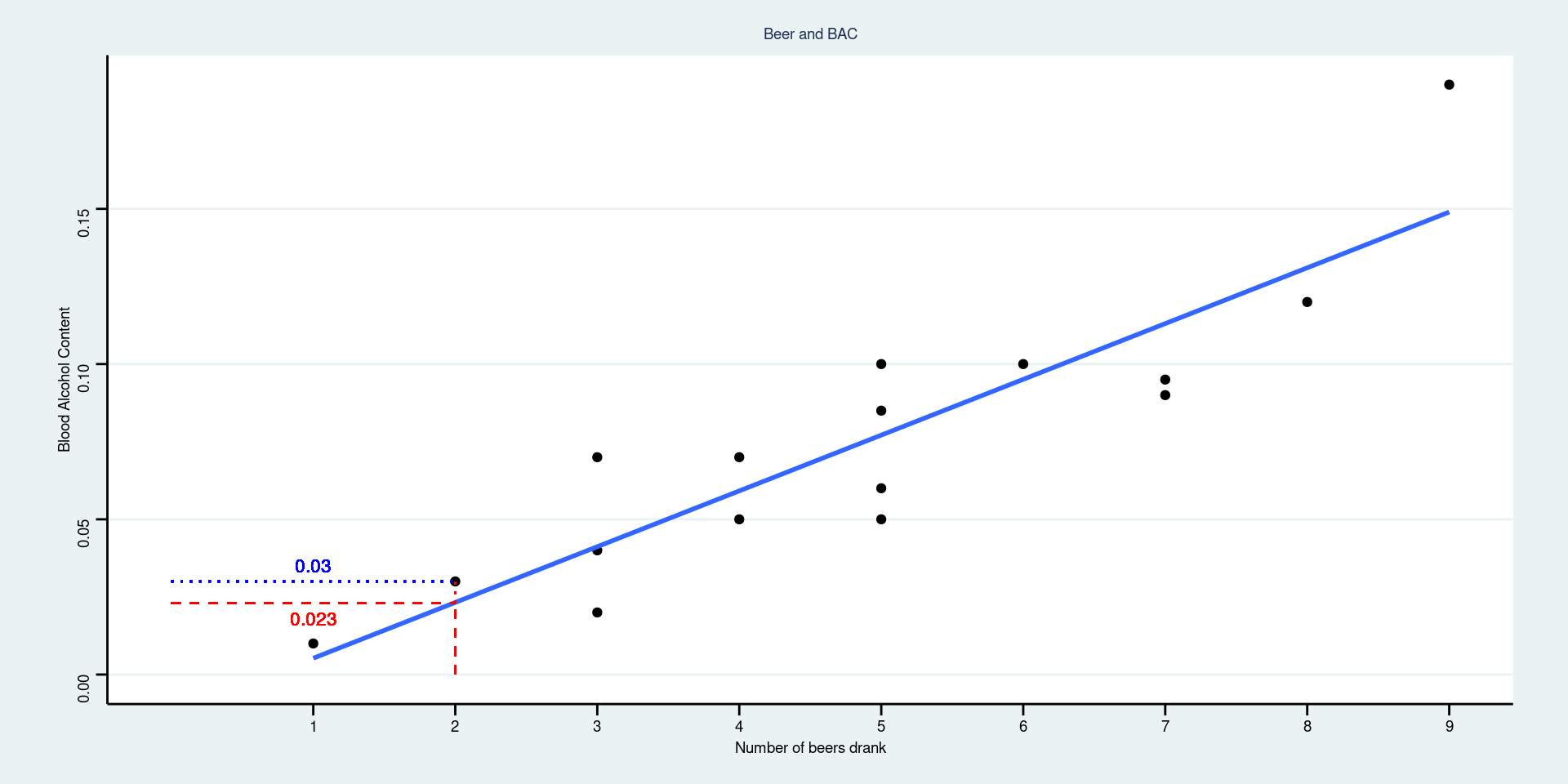
If your friend drank 2 beers, what is your best guess at their BAC after 30 minutes? \[\widehat{BAC} = -0.0127 + 0.0180(2) = 0.023\]

Regressing BAC on number of beers

Find the residual for the student in the dataset who drank 2 beers and had a BAC of 0.03. The residual is about \(y - \hat{y} = 0.03 - 0.023 = 0.007\)

R-squared

R-squared is proportion (or percentage) of variability observed in the response y which can be explained by the explanatory variable x.

\(R^2 = r^2\) in simple linear regression model (One explanatory variable)]

BAC : \(R^2 = 0.7998\)

The number of beers consumed explains about 80.0% of the observed variation in BAC
What factors (variables) besides number of beers drank might explain the other roughly 20% of variation in BAC?

R-squared

Called Multiple R-squared in the summary output

summary(bac.lm)


Call:
lm(formula = BAC ~ Beers, data = bac)

Residuals:
      Min        1Q    Median        3Q       Max 
-0.027118 -0.017350  0.001773  0.008623  0.041027 

Coefficients:
             Estimate Std. Error t value Pr(>|t|)    
(Intercept) -0.012701   0.012638  -1.005    0.332    
Beers        0.017964   0.002402   7.480 2.97e-06 ***
---
Signif. codes:  0 '***' 0.001 '**' 0.01 '*' 0.05 '.' 0.1 ' ' 1

Residual standard error: 0.02044 on 14 degrees of freedom
Multiple R-squared:  0.7998,    Adjusted R-squared:  0.7855 
F-statistic: 55.94 on 1 and 14 DF,  p-value: 2.969e-06

Adding a categorical variable (confounding variable)

library(ggplot2)
ggplot(bac, aes(x = Beers, y = BAC, color = Sex)) + 
  geom_point()

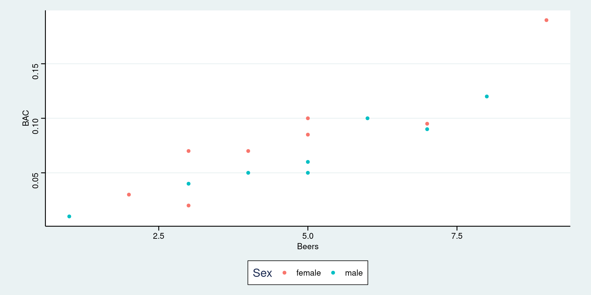
Visually split the data by Sex. Potentially find different trends.

Adding a categorical variable (confounding variable)

library(ggplot2)
ggplot(bac, aes(x = Beers, y = BAC, color = Sex)) + 
  geom_point() + 
  geom_smooth(method = "lm", se = FALSE)

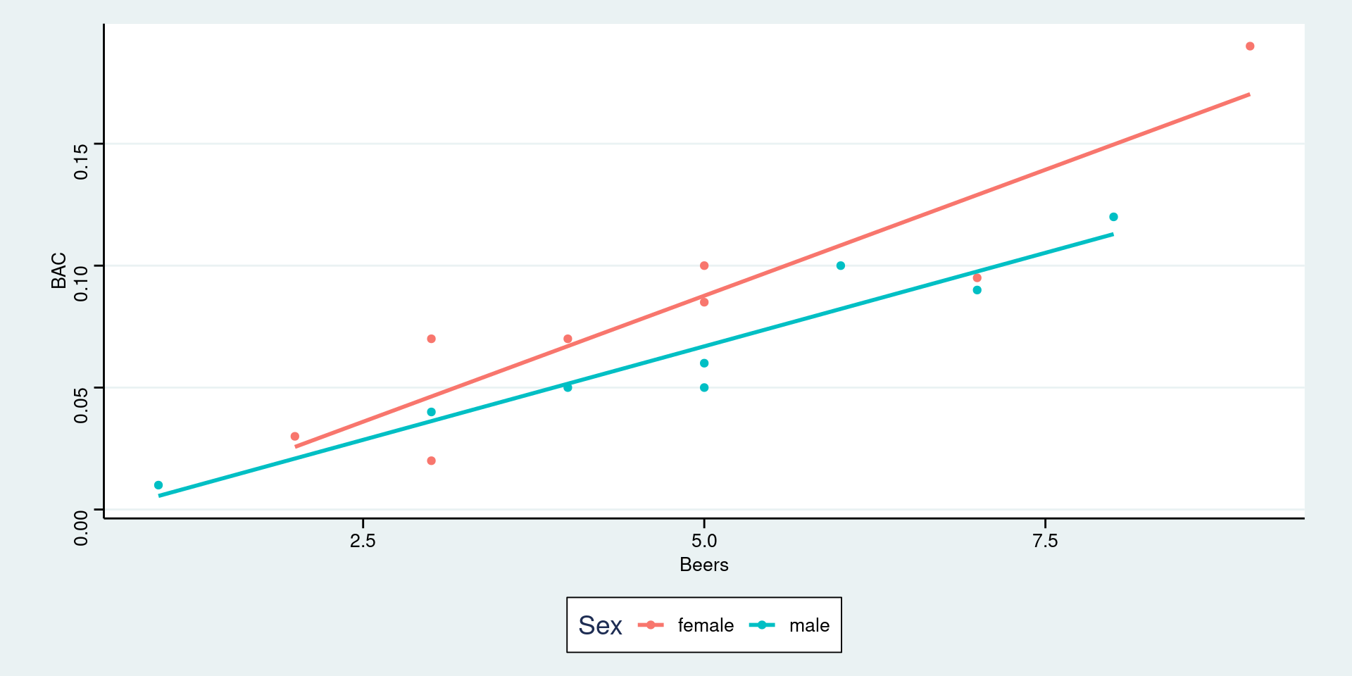
Visually infer difference in Sex in terms of correlation or intercepts

Adding a categorical variable: stats by group

Can also use filter function available under dplyr package to divide responses into the groups of interest

library(dplyr)
table(bac$Sex)


female   male 
     8      8

bac_female <- filter(bac, Sex == "female")
bac_male <- filter(bac, Sex == "male")

cor(bac_female$BAC,bac_female$Beers)

[1] 0.9181408

cor(bac_male$BAC,bac_male$Beers)

[1] 0.9549385

Outliers: Average SAT by state

library(dplyr)
sat <- read.csv("https://math.carleton.edu/Stats215/RLabManual/sat.csv")
sat.MW <- filter(sat, region == "Midwest") # just MW states
cor(sat.MW$math, sat.MW$verbal)

[1] 0.9731605

sat.lm <- lm(math ~ verbal, data=sat.MW)
sat.lm


Call:
lm(formula = math ~ verbal, data = sat.MW)

Coefficients:
(Intercept)       verbal  
    -23.584        1.047

summary(sat.lm)$r.squared

[1] 0.9470413

Correlation = 0.9732, Regression Slope = 1.0469, R-squared = 94.7%

Outliers: Average SAT by state, excluding Indiana and Ohio

library(dplyr)
# Find the rows where 'verbal' is less than 550 using filter
filtered_data <- filter(sat.MW, verbal < 550)
# Exclude data corresponding to specific indices and calculate correlation
filtered_sat_MW <- sat.MW %>%  slice(-c(2, 10))
cor_result <- cor(filtered_sat_MW$math, filtered_sat_MW$verbal)

sat.lm.noIO <- lm( math ~ verbal, data=sat.MW, subset = -c(2,10))
sat.lm.noIO


Call:
lm(formula = math ~ verbal, data = sat.MW, subset = -c(2, 10))

Coefficients:
(Intercept)       verbal  
     6.1453       0.9956

summary(sat.lm.noIO)$r.squared

[1] 0.7166161

Please download the Class-Activity-6 template from moodle and go to class helper web page

20:00

Two Quantitative Variables: Association

Describing associations between two quantitative variables

Example: Associations in Car dataset

Direction

Correlation Coefficients

R-code:

Car Correlations

Linear Regression

Residuals

Presence of Outliers

Regression line of Blood Alcohol Content (BAC) data

Regression line of Blood Alcohol Content (BAC) data

Regressing BAC on number of beers

Regressing BAC on number of beers

Regressing BAC on number of beers

R-squared

R-squared

Adding a categorical variable (confounding variable)

Adding a categorical variable (confounding variable)

Adding a categorical variable: stats by group

Outliers: Average SAT by state

Outliers: Average SAT by state, excluding Indiana and Ohio

Group Activity 1