Sampling Distribution and Bootstrap
STAT 120
Statistical Inference
Statistical inference is the process of drawing conclusions about the entire population based on information in a sample.
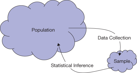
Statistical Inference
Motivating Example 1
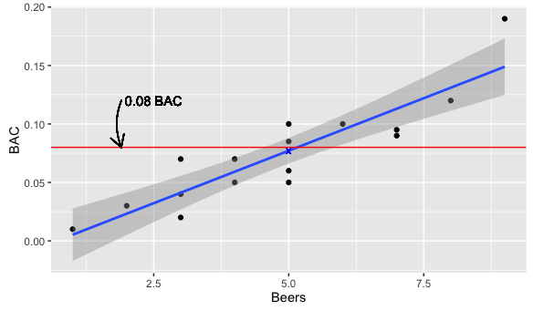
Regression line of Bood alcohol content (BAC) Vs. number of beers
Can you drink 5 beers and stay under the 0.08 limit?
Motivating Example 2
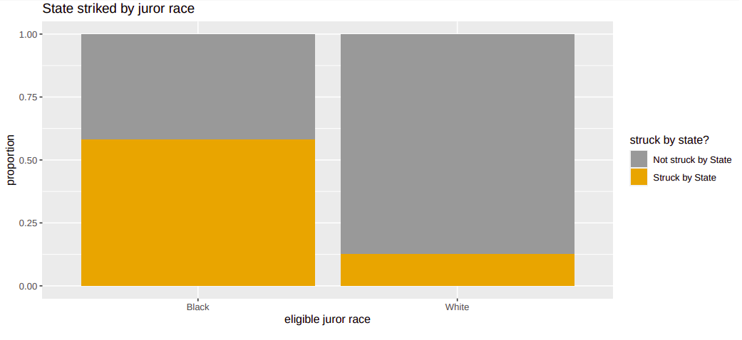
Striking rates by race
Do the observed differences in strike rates between black and white eligible jurors indicate a potential bias, or are the differences just due to chance?
Group Activity 1
05:00
Recall: Gettysburg Address
The standard error for the average word size in a random sample of 10 words is closest to
- 0.5
- 0.7
- 1.0
- 1.5
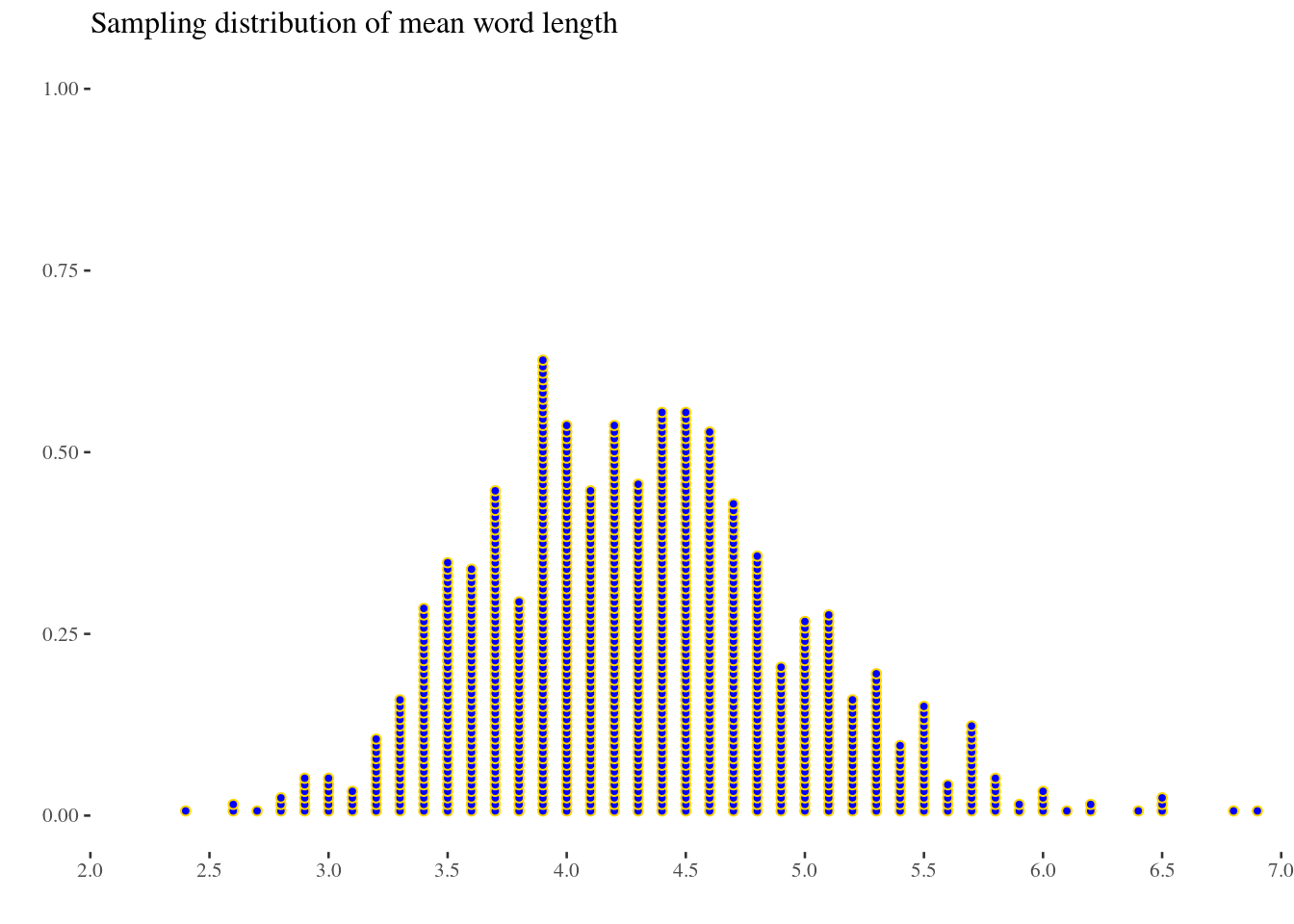
Sample Size Matters!
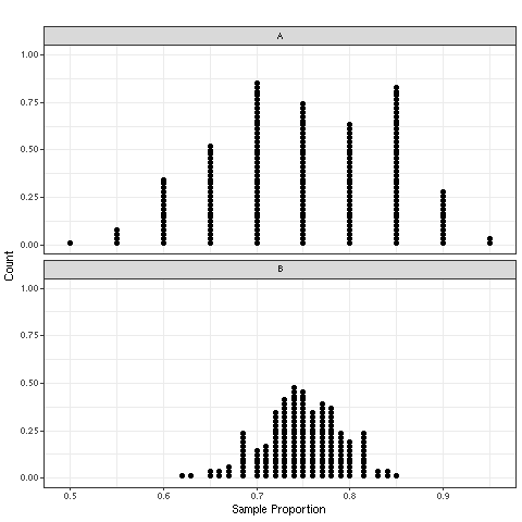
Random Vs. Non-random
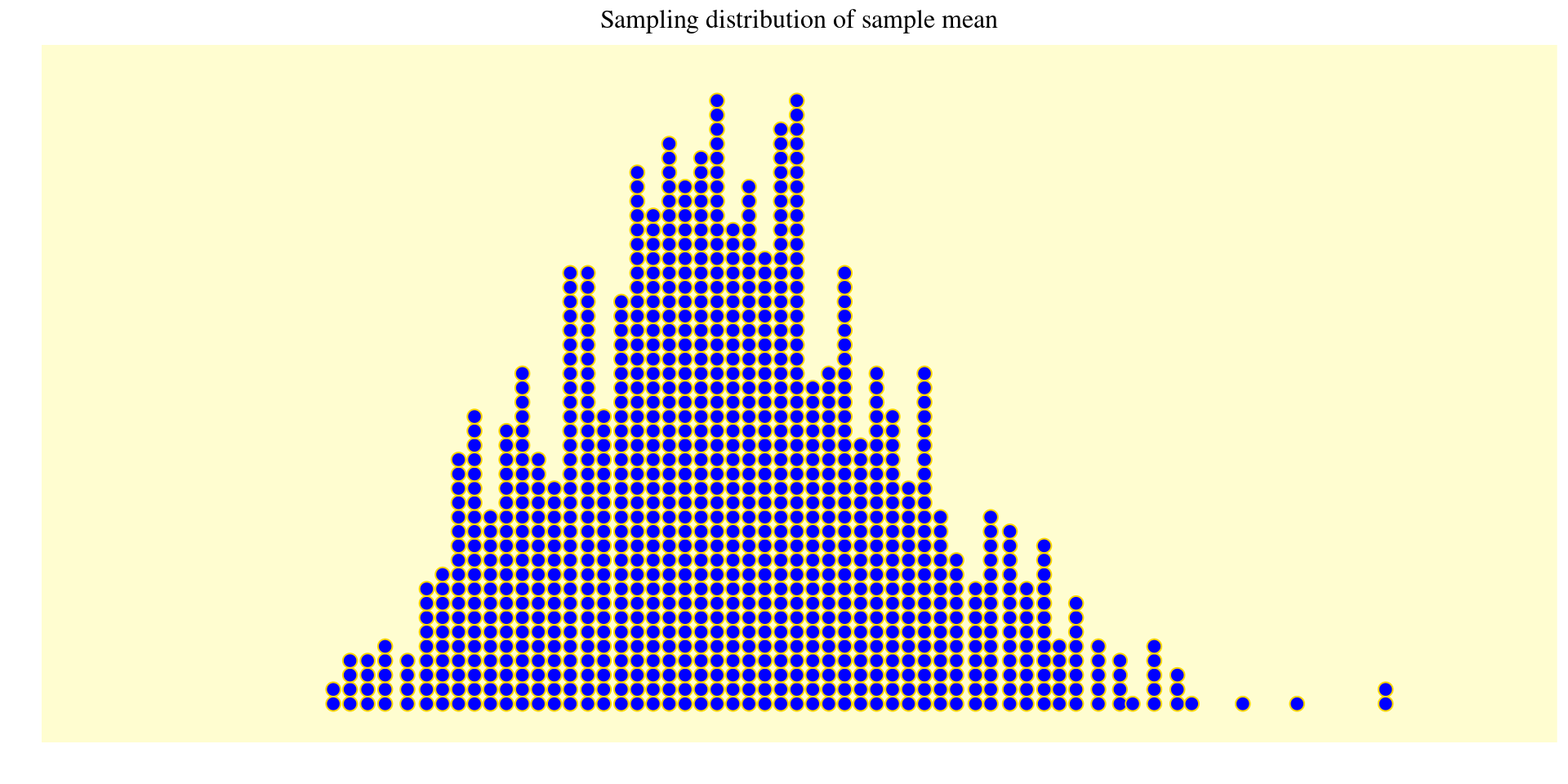
Samples of size 5 are taken from a large population with population mean 8, and the sampling distributions for the sample means are shown. Dataset A (top) and Dataset B (bottom) were collected using different sampling methods. Which dataset (A or B) used random sampling?
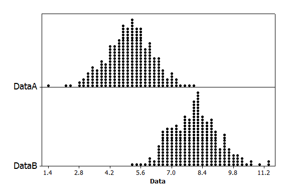
Random Vs. non-random data distribution
Bootstrap
Bootstrap: Sample with replacement from the original sample, using the same sample size.
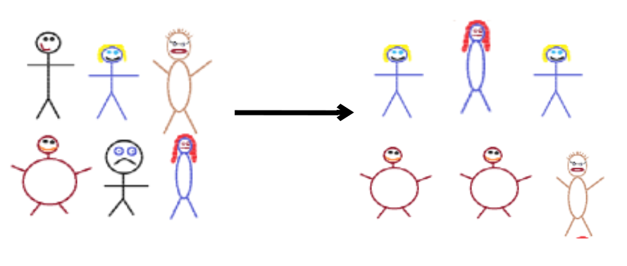
Original sample (left) to bootstrap sample (right)
Bootstrap
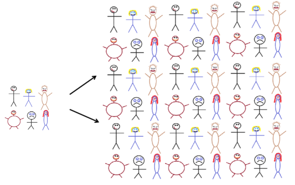
Original sample (left) to population (right)
Creating a bootstrap sample is the same as using the data simulate a “population” that contains an infinite number of copies of the data.
Group Activity 2

- Please download the Class-Activity-7 template from moodle and go to class helper web page
20:00