(a). If the results of a test for ESP are statistically discernible, what does that mean in terms of ESP?
Click for answer
Answer:
It means we can conclude that \(p > 0.2\) and that the sample results were so strong that we can conclude that ESP does exist and get more right than would be expected by random chance.
(b). If the results are not statistically discernible, what does that mean in terms of ESP?
Click for answer
Answer:
The sample results are inconclusive. People may or may not have ESP. Sample results could be just random chance.
Problem 2: Sleep or Caffeine for Memory
In an experiment, 24 students were given words to memorize, then were randomly assigned to take a 90 minute nap or take a caffeine pill (12 in each group). They were then tested on their recall ability. We test to see if the sample provides evidence that there is a difference in mean number of words people can recall depending on whether they take a nap or have some caffeine. The hypotheses are:
The sample mean difference is \(\bar{x}_S - \bar{x}_C = 3\). We want to know if this difference in sample means is statistically discernible.
(a) Explain how to generate a randomization distribution for \(\bar{x}_S - \bar{x}_C\) that is consistent with \(H_0: \mu_S - \mu_C = 0\).
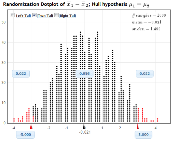
Click for answerAnswer: We could randomly reassign the treatment to the study participants since, under the null, their recall abilities would be the same under either treatment. For each reassignment, we recomputed the sample mean difference and plot it in the dotplot shown below
(b) Navigate to the Statkey website.
Select the Test for Difference in Means option under Randomization Hypothesis Tests. Change the data set from Leniency and Smiles to Sleep Caffeine Words. Note that the original sample data has a sample mean difference of 3 words.
Generate 1 Sample from this null randomization distribution. What is the difference in the average word recall of the two groups in this sample? Repeat this a couple of times.
Generate 1000 Samples a few of times (get at least 3000 resamples). How unusual is getting a difference in means of 3 or more words?
(c) Compute the randomization p-value
Select the Two-Tail button at the top of the plot. Change the positive x-axis value to the observed difference of 3.0. The p-value is 2 times the proportion of resamples that have a difference of 3 or above. What is the p-value?
Example 2c
Click for answerAnswer: We see in the image that the proportion in the tail beyond the sample statistic of 3.0 is 0.022. Because this is a two-tail test, we have to account for both tails, so the p-value is 2(0.022) = 0.044.
(d) Interpret + Conclusion
Interpret the p-value. Does the p-value support the alternative hypothesis (do you think difference of means of 3 is statistically discernible) or is it inconclusive? Explain.
Click for answerAnswer: We would see a difference of at least 3 words recalled, on average, in about 4.4% of all possible samples if the influence of sleep and caffeine on recall was the same The results show some evidence of statistical significance, meaning that the caffeine and sleep may have some difference effects on word recall ability.
(e) Redo in Rstudio
First get the data from the Lock website and check important summary stats:
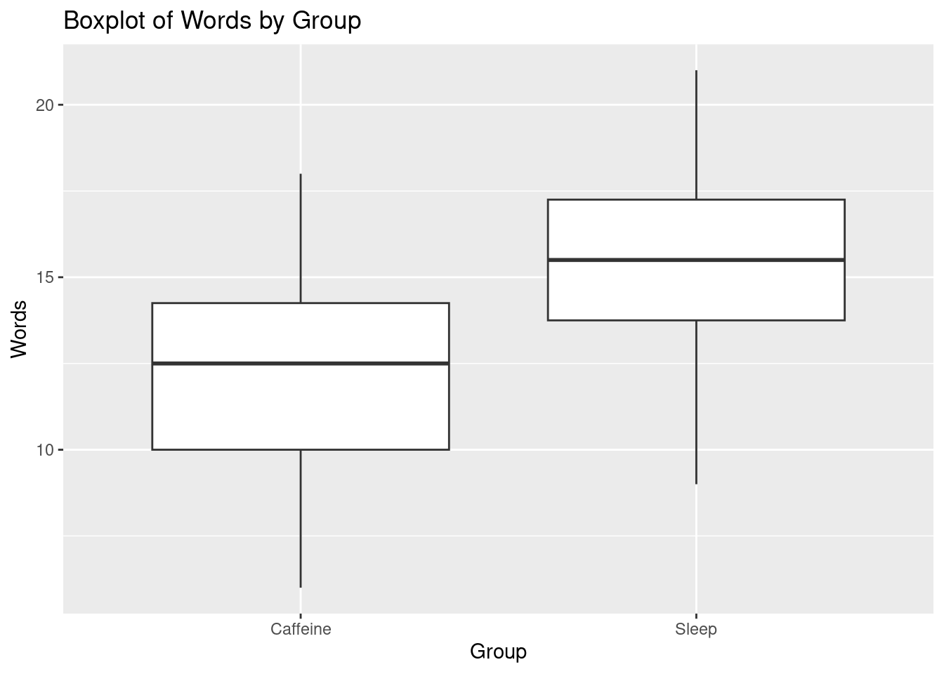
SleepCaffeine <-read.csv("http://math.carleton.edu/Stats215/Textbook/SleepCaffeine.csv")# Create a boxplot using ggplot2library(ggplot2)ggplot(SleepCaffeine, aes(x = Group, y = Words)) +geom_boxplot() +labs(title ="Boxplot of Words by Group")
# Summary statistics using dplyr for 'Words'library(dplyr)SleepCaffeine %>%group_by(Group) %>%summarize(min =min(Words, na.rm =TRUE),q1 =quantile(Words, 0.25, na.rm =TRUE),median =median(Words, na.rm =TRUE),mean =mean(Words, na.rm =TRUE),q3 =quantile(Words, 0.75, na.rm =TRUE),max =max(Words, na.rm =TRUE),sd =sd(Words, na.rm =TRUE) ) %>% knitr::kable(caption="Summary Statistics of Words Recalled by Treatment Group")
Summary Statistics of Words Recalled by Treatment Group
Group
min
q1
median
mean
q3
max
sd
Caffeine
6
10.00
12.5
12.25
14.25
18
3.545163
Sleep
9
13.75
15.5
15.25
17.25
21
3.306330
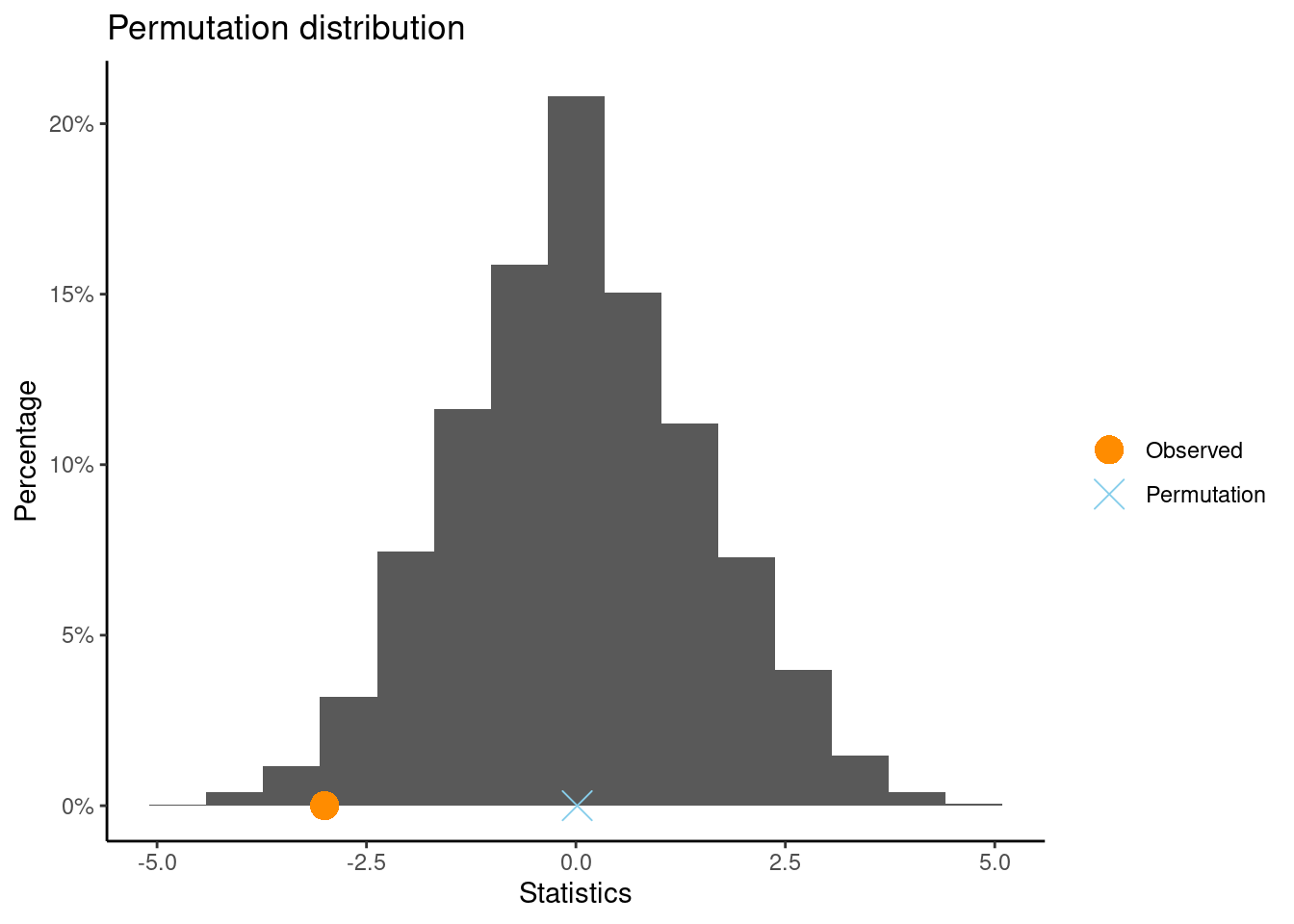
Then load the CarletonStats package and run the permTest(y ~ x, data=) command where y is your quantitative (or 0/1 coded) response and x defines the two groups you are comparing.
    ** Permutation test **

 Permutation test with alternative: two.sided
 Observed statistic
  Caffeine :  12.25      Sleep :  15.25
 Observed difference: -3

 Mean of permutation distribution: 0.01573
 Standard error of permutation distribution: 1.49817
 P-value:  0.0492

    *-------------*
Why is the observed difference reported as -3?
Click for answerAnswer: The difference is computed alphabetically: Caffeine minus Sleep so the difference in now -3 instead of +3.
What is the p-value? Is it the same as the Statkey p-value? The same as your neighbors p-value? Why not?
Click for answerAnswer: The p-value is around 5%. Any difference between Statkey, neighbors or different runs of the permTest command stem from the fact that different resamples are obtained each time a randomization distribution is generated. There may be some small (inconsequential) difference in p-values due to this.
Problem 3: Resident vs Non-resident Tuition
The lab manual data set Tuition2006 is a random sample of state colleges and universities in the U.S. We want to know if the average tuition charged to non-residents is higher than residents for all state colleges and universities:
Read in the data. Note that each case (school) has a response value for the resident and non-resident tuition variables. This makes this a paired data example. Contrast this with the word recall example in which each case (student) only had one response (word recall) and treatment (caffeine/sleep).
Summary Statistics of Difference in Residential and Non-residential Tuition
min
q1
median
mean
q3
max
sd
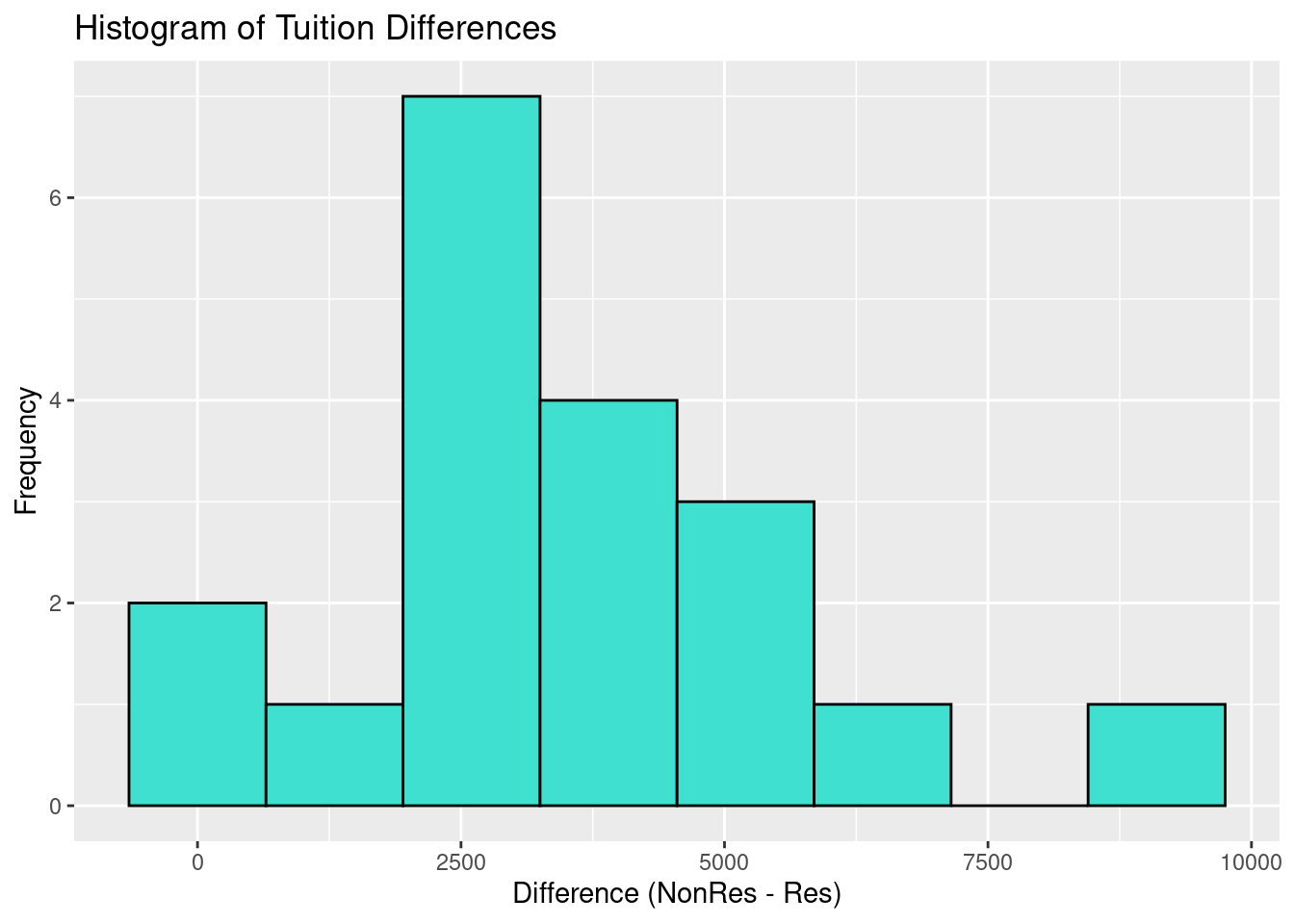
200
2650
3100
3584.211
4500
9300
2073.447
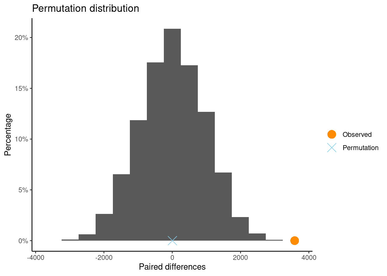
# Histogram of 'diff'ggplot(tuition, aes(x = diff)) +geom_histogram(binwidth =1300, fill ="turquoise", color ="black") +labs(title ="Histogram of Tuition Differences", x ="Difference (NonRes - Res)", y ="Frequency")
What is the average difference in tuition costs?
Click for answerAnswer: The observed mean difference is $3584
Is this observed mean difference statistically significant? To test use the command permTestPaired:
set.seed(123)permTestPaired(NonRes ~ Res,data = tuition, alt ="greater")
    ** Permutation test **

 Permutation test with alternative: greater
 Observed mean
  NonRes :  2821.053     Res :  6405.263
 Observed difference: 3584.211

 Mean of permutation distribution: 4.69679
 Standard error of permutation distribution: 950.3981
 P-value:  1e-04

    *-------------*
The alt of greater was used because the function permTestPaired(A ~ B) computes paired differences as “A” minus “B”.
What is the p-value for this test?
Click for answer
Answer: Less than 0.0001
Is this observed mean difference statistically significant?
Click for answer
Answer: Yes, an observed mean difference of at least $3584 would rarely occur just by chance which provides us strong evidence that the mean tuition amount of non-residents is higher than residents in the population of state colleges and universities (in 2006).
Problem 4: Evaluating Drugs to Fight Cocaine Addition
In a randomized experiment on treating cocaine addiction, 48 cocaine addicts who were trying to quit were randomly assigned to take either desipramine (a new drug), or Lithium (an existing drug). The response variable is whether or not the person relapsed (which means the person was unable to break out of the cycle of addiction and returned to using cocaine.) We are testing to see if desipramine is better than lithium at treating cocaine addiction. The results are shown in the two-way table.
\
Relapse
No Relapse
total
Desipramine
10
14
24
Lithium
18
6
24
(a) Using \(p_D\) for the true proportion of desipramine users who relapse and \(p_L\) for the true proportion of lithium users who relapse, write the null and alternative hypotheses.
(b) Compute the appropriate sample statistic needed to assess the hypotheses above.
Click for answer
Answer: We see that \(\hat{p}_D = \dfrac{10}{24} = 0.417\) and \(\hat{p}_L = \dfrac{18}{24} = 0.75\) so we have \(\hat{p}_D -\hat{p}_L = 0.417 - 0.75 = -0.333\). Be sure to compute the difference since we need one number (observed difference) to test the hypotheses, not two separate numbers. You could also compute the difference as \(L-D\) and get +0.333.
(c) How might we compute a randomization sample for this data?
Click for answer
Answer: Since drug doesn’t matter, we combine all 48 patients together and see that 28 relapsed and 20 didn’t. To see what happens by random chance, we randomly divide them into two groups and compute the difference in proportions of relapses between the two groups. The difference in proportions is the statistic.
(d) Navigate to the Statkey website.
Select the Test for Difference in Proportions option under Randomization Hypothesis Tests. Click Edit Data and let Group 1 be “Desipramine” and 2 be “Lithium”, enter relapse counts of 10 and 18 and sample sizes of 24. Check that the null hypothesis matches yours in (a). Generate a couple thousand samples. Describe the resulting distribution. Where is it centered?
Click for answer
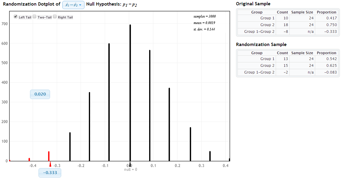
Answer: The resulting distribution, shown in Figure 1, will be bell-shaped and centered at the value from the null hypothesis, which is zero.
Example 4d
(e) Compute and interpret the p-value for this test.
Click for answer
Answer: This is a left-tail test when computing the difference as D - L, and we see on StatKey that the p-value (proportion of randomization samples with a difference -.333 or smaller) is about 2 (Figure 1). About 2% of the time we would see at least 33% fewer relapse cases using despramine than lithium just due to chance if there was no difference in the relapse rates of the two treatments.
Note the two key features of this “in context” interpretation of 2%: it assumes that the null is true (no treatment difference) and it uses the observed statistic (data) used to compute the p-value (rate of despramine relapse is .33 below the rate of lithium).
(f) Make a formal decision (reject or not) using a 5% significance level, then restate your conclusion in context for the problem (do not use words like “reject” or “hypothesis”).
Click for answer
Answer: We reject the null hypothesis since the p-value of 2% is less than 5%. We can conclude that despramine is better at helping people kick the cocaine habit. Note the “in context” conclusion: Just state your conclusion in english, no need to talk about the value of the p-value or “just by chance.”
(h) Use Statkey to compute and interpret a 95% bootstrap confidence interval for the difference in the relapse proportion for the two treatments. Explain how this CI agrees with your test conclusion in (f).
Click for answer
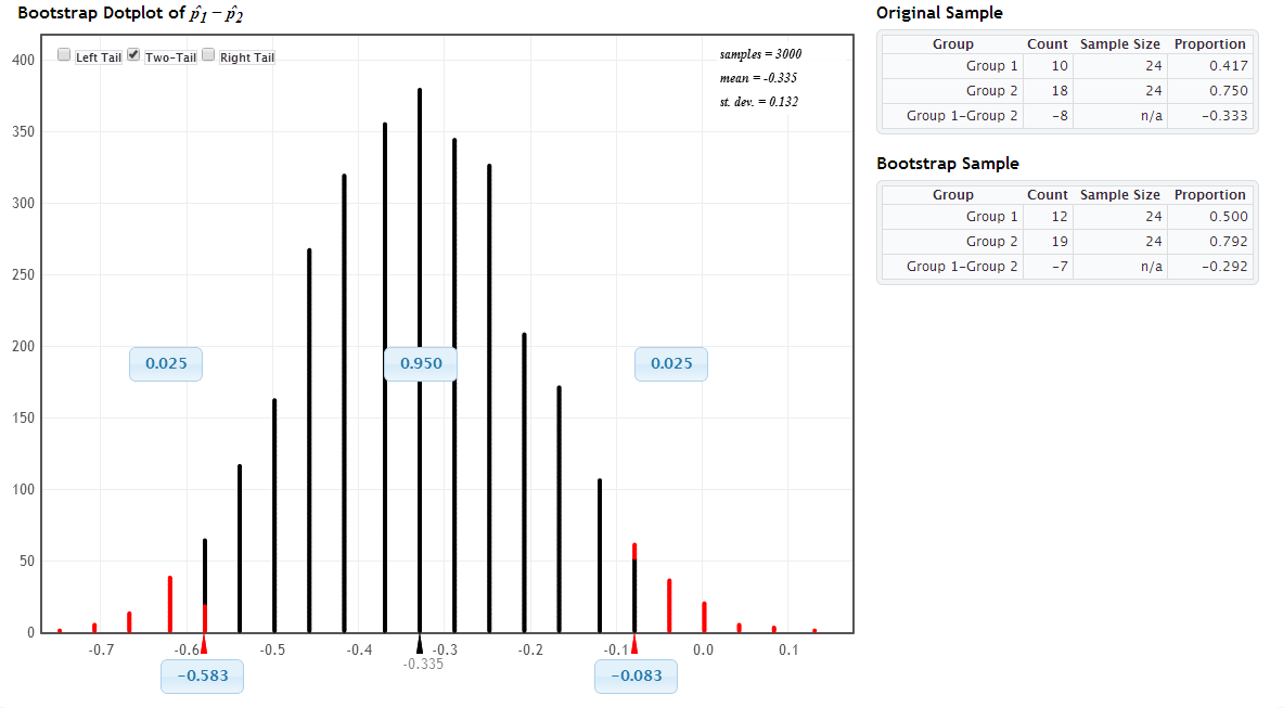
Answer: I am 95% confident that the relapse rate for despramine will be between 8.3 to 58.3 percent less than the relapse rate for lithium. This completely agrees with the test conclusion that despramine is a better treatment for cocaine addiction. (Figure 2 shows the bootstrap distribution that is centered at the sample difference of -0.333.)