library(ggplot2)
sleep <- read.csv("http://math.carleton.edu/Stats215/Textbook/SleepStudy.csv")
ggplot(sleep, aes(x=AverageSleep)) +
  geom_histogram(fill="steelblue", bins = 30) +
  labs(title = "Distribution of Sleep Hours", x = "Hours of Sleep")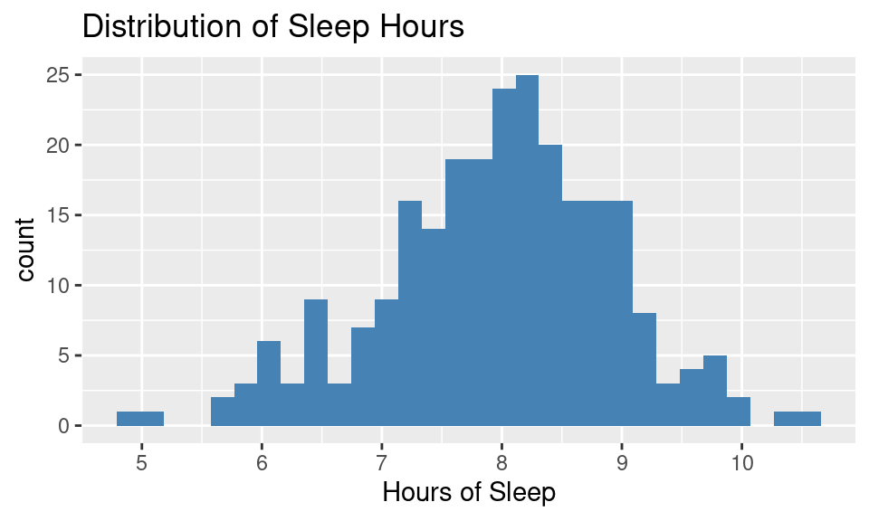
This histogram shows the distribution of hours or sleep per night for a large sample of students.
library(ggplot2)
sleep <- read.csv("http://math.carleton.edu/Stats215/Textbook/SleepStudy.csv")
ggplot(sleep, aes(x=AverageSleep)) +
geom_histogram(fill="steelblue", bins = 30) +
labs(title = "Distribution of Sleep Hours", x = "Hours of Sleep")
Answer: The mean is around 8 hours
Answer: Most of the data is between about 6 and 10, with a mean around 8 (due to the roughly symmetric distribution). So two standard deviations is about 2 hours of sleep, making one standard deviation about 1 hours of sleep.
Let’s check the rule! Here are the actual mean and SD:
mean(sleep$AverageSleep)[1] 7.965929sd(sleep$AverageSleep)[1] 0.9648396The ACT test has a population mean of 21 and standard deviation of 5. The SAT has a population mean of 1500 and a standard deviation of 325. You earned 28 on the ACT and 2100 on the SAT.
Answer:
z_ACT <- (28 - 21) / 5
z_SAT <- (2100 - 1500) / 325
z_ACT
[1] 1.4z_SAT[1] 1.846154Answer:
ACT_lower <- 21 - 2 * 5
ACT_upper <- 21 + 2 * 5
SAT_lower <- 1500 - 2 * 325
SAT_upper <- 1500 + 2 * 325
c(ACT_lower, ACT_upper)
[1] 11 31c(SAT_lower, SAT_upper)[1] 850 2150For the given vector of observations indicate whether the resulting data appear to be symmetric, skewed to the right, or skewed to the left.
(2, 10, 15, 20, 69, 34, 23, 2, 45)
my_vector <- c(2, 10, 15, 20, 69, 34, 23, 2, 45)
summary(my_vector)
Min. 1st Qu. Median Mean 3rd Qu. Max.
2.00 10.00 20.00 24.44 34.00 69.00 Answer: Skewed right. It has a longer right tail than left since max -Q3 >> Q1 - min
ggplot(data.frame(x=my_vector), aes(x)) + geom_boxplot()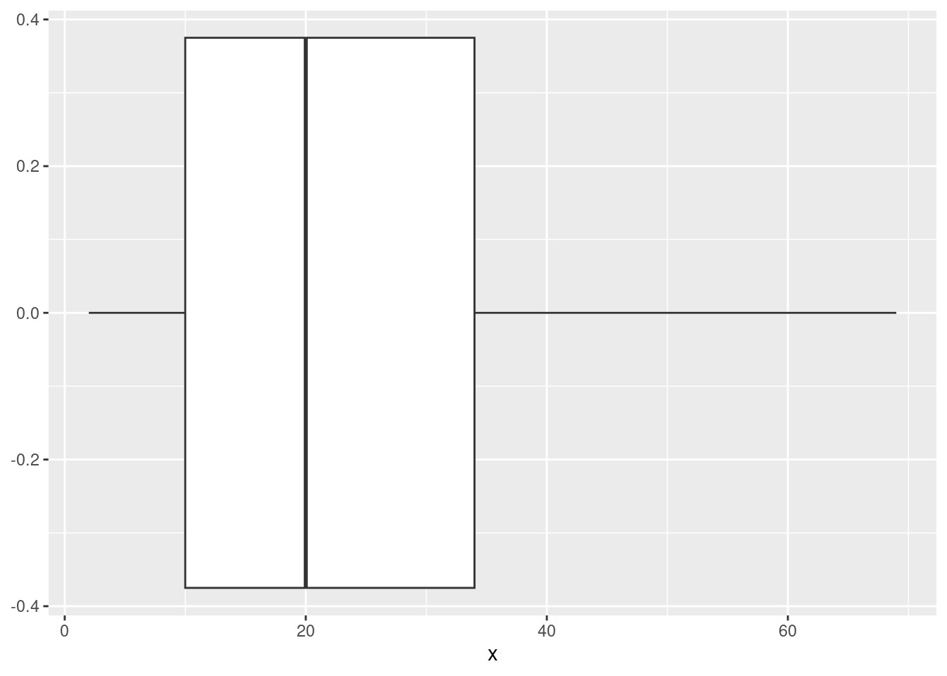
This boxplot shows the number of hot dogs eaten by the winners of Nathan’s Famous hot dog eating contests from 2002-2011.
hotdogs <- read.csv("https://raw.githubusercontent.com/deepbas/statdatasets/main/HotDogs.csv")
ggplot(hotdogs, aes(x = "", y = HotDogs)) +
  geom_boxplot() +
labs(title = "Number of Hot Dogs Consumed", y = "Number of Hot Dogs") 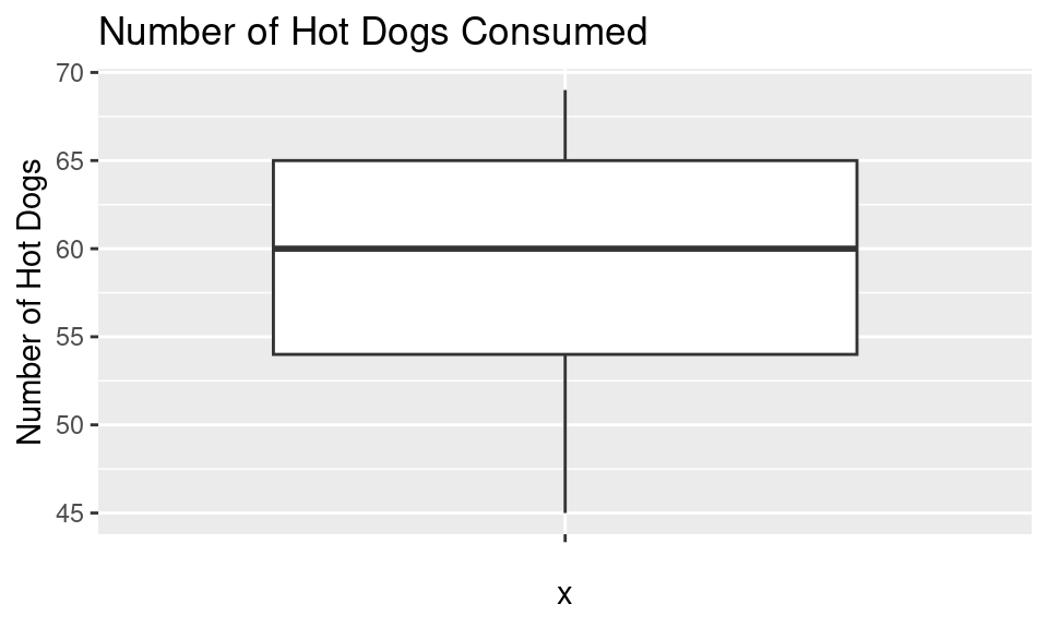
Answer:
hotdog_q1 <- quantile(hotdogs$HotDogs, 0.25); hotdog_q125%
54 hotdog_q3 <- quantile(hotdogs$HotDogs, 0.75); hotdog_q375%
65 hotdog_iqr <- IQR(hotdogs$HotDogs); hotdog_iqr[1] 11lower_fence <- hotdog_q1 - 1.5 * hotdog_iqr; lower_fence 25%
37.5 upper_fence <- hotdog_q3 + 1.5 * hotdog_iqr; upper_fence 75%
81.5 library(dplyr)
outliers <- filter(hotdogs, HotDogs < lower_fence | HotDogs > upper_fence)
outliers[1] Year HotDogs
<0 rows> (or 0-length row.names)Let’s visit the WorldGross analysis from the Hollywood movies data set:
movies <- read.csv("https://raw.githubusercontent.com/deepbas/statdatasets/main/HollywoodMovies2011.csv")WorldGross.Answer:
ggplot(movies, aes(x = WorldGross, y = "")) +
  geom_boxplot() +
labs(title = "World Gross of Hollywood Movies", x = "World Gross (in millions)", y ="") 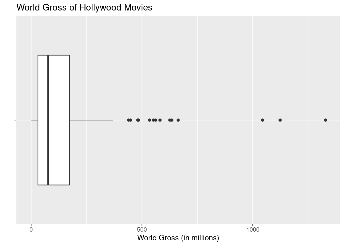
How many movies are identified as outliers for world gross?
Use the boxplot outlier rule to find the “fence” (cutoff) between an outlier and non-outlier for WorldGross. Then determine the value (of WorldGross) that the upper “whisker” (non-outlier) extends to.
Answer:
library(tidyr)
movies_no_na <- drop_na(movies)   # drop missing values
q1_world_gross <- quantile(movies_no_na$WorldGross, 0.25)
q3_world_gross <- quantile(movies_no_na$WorldGross, 0.75)
iqr_world_gross <- IQR(movies_no_na$WorldGross)
lower_fence_world_gross <- q1_world_gross - 1.5 * iqr_world_gross
upper_fence_world_gross <- q3_world_gross + 1.5 * iqr_world_gross

outliers <- filter(movies_no_na, WorldGross < lower_fence_world_gross | WorldGross > upper_fence_world_gross)
outliers
Movie LeadStudio
1 Harry Potter and the Deathly Hallows Part 2 Warner Bros
2 The Hangover Part II Legendary Pictures
3 Twilight: Breaking Dawn Independent
4 Transformers: Dark of the Moon DreamWorks Pictures
5 Rio 20th Century Fox
6 Rise of the Planet of the Apes 20th Century Fox
7 The Smurfs Sony Pictures Animation
8 Kung Fu Panda 2 DreamWorks Animation
9 Pirates of the Caribbean:\nOn Stranger Tides Disney
10 Mission Impossible Paramount
11 Sherlock Holmes 2 Warner Bros
12 Thor Disney
13 Cars 2 Pixar
RottenTomatoes AudienceScore Story Genre TheatersOpenWeek
1 96 92 Rivalry Fantasy 4375
2 35 58 Comedy Comedy 3615
3 26 68 Love Romance 4061
4 35 67 Quest Action 4088
5 71 73 Quest Animation 3826
6 83 87 Revenge Action 3648
7 23 50 Fish Out Of Water Animation 3395
8 82 80 Rivalry Animation 3925
9 34 61 Quest Action 4155
10 93 86 Pursuit Action 3448
11 60 79 Pursuit Action 3703
12 77 80 Monster Force Action 3955
13 38 56 Fish Out Of Water Animation 4115
BOAverageOpenWeek DomesticGross ForeignGross WorldGross Budget Profitability
1 38672 381.01 947.10 1328.111 125 10.624888
2 23775 254.46 327.00 581.464 80 7.268300
3 34012 260.80 374.00 634.800 110 5.770909
4 23937 352.39 770.81 1123.195 195 5.759974
5 10252 143.62 341.02 484.634 90 5.384822
6 15024 176.70 304.52 481.226 93 5.174473
7 10489 142.61 419.54 562.158 110 5.110527
8 12142 165.25 497.78 663.024 150 4.420160
9 21697 241.07 802.80 1043.871 250 4.175484
10 8672 197.80 336.70 534.500 145 3.686207
11 10704 179.04 261.00 440.040 125 3.520320
12 16618 181.03 267.48 448.512 150 2.990080
13 16072 191.45 360.40 551.850 200 2.759250
OpeningWeekend
1 169.19
2 85.95
3 138.12
4 97.85
5 39.23
6 54.81
7 35.61
8 47.66
9 90.15
10 29.55
11 39.63
12 65.72
13 66.14movies_no_outliers that contains only the rows from movies_no_na where the WorldGross values are within the range defined by the lower and upper fences.Answer:
library(dplyr)
movies_no_outliers <- filter(movies_no_na, WorldGross >= lower_fence_world_gross & WorldGross <= upper_fence_world_gross)We can compare boxplots of WorldGross across Genre categories:
ggplot(movies, aes(x = Genre, y = WorldGross)) +
  geom_boxplot() +
  labs(title = "World Gross by Genre", x = "Genre", y = "World Gross (in millions)") +
  theme(axis.text.x = element_text(angle = 45, hjust = 1))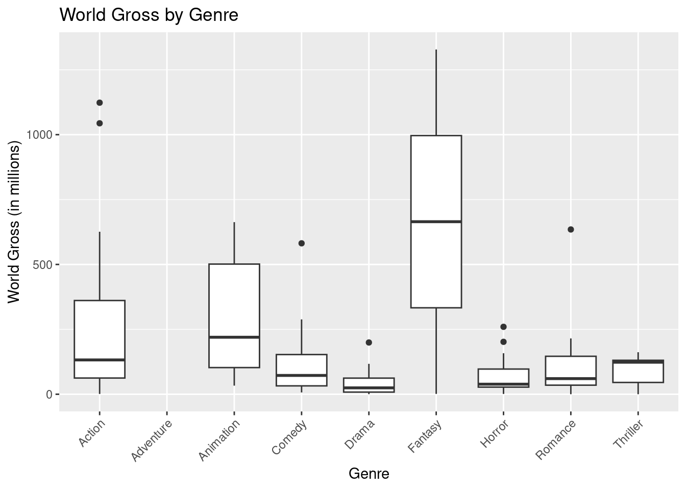
WorldGross and Genre?WorldGross and Genre?