(0.67 - 0.5)/0.021[1] 8.095238In a study, we find that 67% of women in a random sample view divorce as morally acceptable. Does this provide evidence that more than 50% of women view divorce as morally acceptable? The standard error for the estimate assuming the null hypothesis is true is 0.021.
Answer: The observed sample proportion is 0.67 with a standard error of 0.021. If the null is true, then we would expect the sampling distribution of the sample mean to be (approximately) normally distributed with a center of 0.50 and SE of 0.021. The standardized score for the sample proportion is then \[ z = \dfrac{\textrm{statistic} - \textrm{null parameter}}{SE} = \dfrac{0.67 - 0.50}{0.021} = 8.10 \] The observed proportion is 8.1 SEs above the hypothesized value of 0.5.
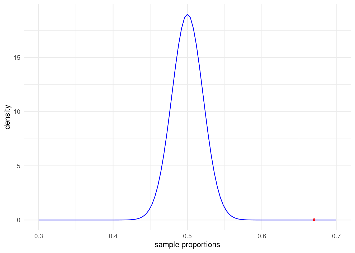
(0.67 - 0.5)/0.021[1] 8.095238Note that the randomization distribution should look roughly like this (with the observed proportion denoted with a red X):
library(ggplot2)

# Create a data frame with a sequence of x values
x_values <- data.frame(x = seq(0.3, 0.7, length.out = 100))

# Use ggplot2 to plot the normal distribution curve and add the red point
ggplot(x_values, aes(x = x)) +
  stat_function(fun = dnorm, args = list(mean = 0.5, sd = 0.021), color = "blue") +
  geom_point(aes(x = 0.67, y = 0), color = "red", shape = "X") +
  xlab("sample proportions") +
  ylab("density") +
  theme_minimal()
Answer: As we can see in the normal plot above, the p-value will be very small because the alternative is looking for big sample proportions. The p-value is the proportion of times we get a sample proportion as big, or bigger than, 0.67; or equivantly, the proportion of times we get a sample proportion that is at least 8.1 SEs above the hypothesized proportion. We would report a p-value that is less than 0.0001.
1-pnorm(8.10,0,1)[1] 2.220446e-16Answer: Without knowing the bootstrap SE, our best guess at it would be from the randomization distribution SE which is given as 0.021. Our 99% confidence interval will look like: \[ statistic \pm z^*SE = 0.67 \pm z^* (0.021) \] The \(z^*\) for a 99% CI corresponds to the 99.5th percentile (90% in middle + 0.5% in the left tail). With \(z^* = 2.576\), we get a 99% confidence interval of 0.616 to 0.724.
qnorm(0.995)[1] 2.5758290.67 - 2.576*0.021[1] 0.6159040.67 + 2.576*0.021[1] 0.724096In the same study described above, we find that 71% of men view divorce as morally acceptable. Use this and the information in the previous example to test whether there is a significant difference between men and women in how they view divorce. The standard error for the difference in proportions under the null hypothesis that the proportions are equal is 0.029.
Answer: Using the same notation as (1a), except denoting male/female populations, we get
\[ H_0: p_f = p_m \ \ H_A: p_f \neq p_m \]
Answer: Suppose we look at the difference \(p_m - p_f\). The observed difference is then 0.04 (0.71 - 0.67). This value is about 1.4 SEs above the hypothesized difference of 0: \[ z = \dfrac{\textrm{statistic} - \textrm{null parameter}}{SE} = \dfrac{(0.71 - 0.67) - 0}{0.029} = 1.379 \]
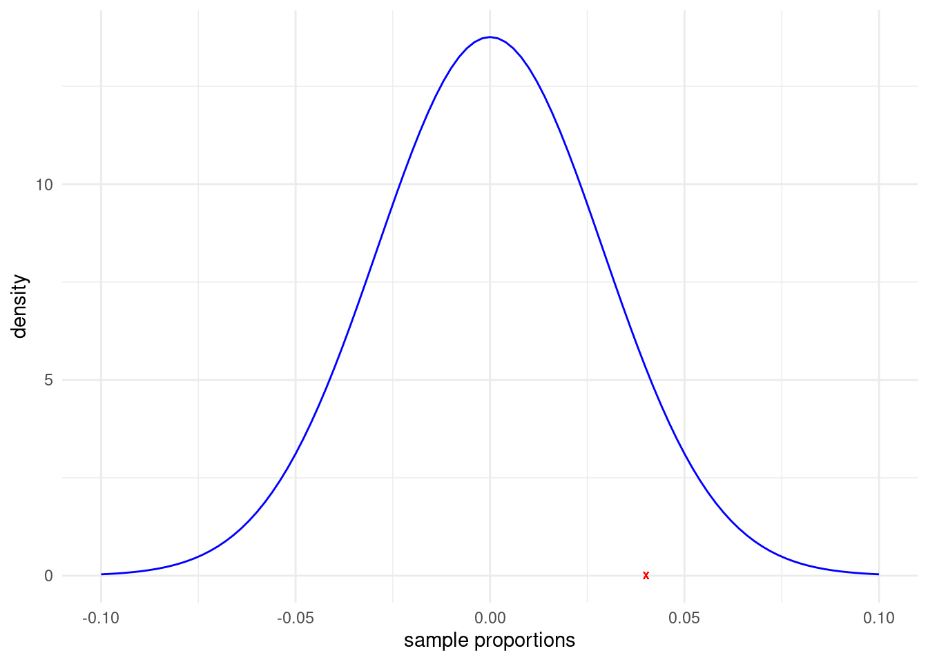
(0.04 - 0)/0.029[1] 1.37931Note that the randomization distribution for the difference in sample proportions should look roughly like this (with the observed proportion difference denoted with a red X):
library(ggplot2)

# Create a data frame with a sequence of x values
x_values <- data.frame(x = seq(-0.1, 0.1, length.out = 100))

# Use ggplot2 to plot the normal distribution curve
ggplot(x_values, aes(x = x)) +
  stat_function(fun = dnorm, args = list(mean = 0, sd = 0.029), color = "blue") +
  geom_point(aes(x = 0.04, y = 0), color = "red", shape = "X") +
  xlab("sample proportions") +
  ylab("density") +
  theme_minimal()
Answer: This is a two-tail test. Since the observed difference is less than 2 SEs away from 0 we know that the (two-tailed) p-value should be bigger than 0.05. We see that the p-value is 2(0.084) = 0.168.
1-pnorm(1.379,0,1) # proportion above z=1.379[1] 0.083947382*(1-pnorm(1.379,0,1)) # p-value for two-sided[1] 0.1678948