Practice Problems 25
Problem 1: Cuckoo Eggs
The common cuckoo does not build its own nest: it prefers to lay its eggs in another birds’ nest. It is known, since 1892, that the type of cuckoo bird eggs are different between different locations. In a study from 1940, it was shown that cuckoos return to the same nesting area each year, and that they always pick the same bird species to be a “foster parent” for their eggs. Over the years, this has lead to the development of geographically determined subspecies of cuckoos. These subspecies have evolved in such a way that their eggs look as similar as possible as those of their foster parents.
The cuckoo dataset contains information on 120 Cuckoo eggs, obtained from randomly selected “foster” nests. For these eggs, researchers have measured the length (in mm) and established the type (species) of foster parent. The type column is coded as follows:
type=1: Hedge Sparrowtype=2: Meadow Pittype=3: Pied Wagtailtype=4: European robintype=5: Tree Pipittype=6: Eurasian wren
The researchers want to test if the type of foster parent has an effect on the average length of the cuckoo eggs.
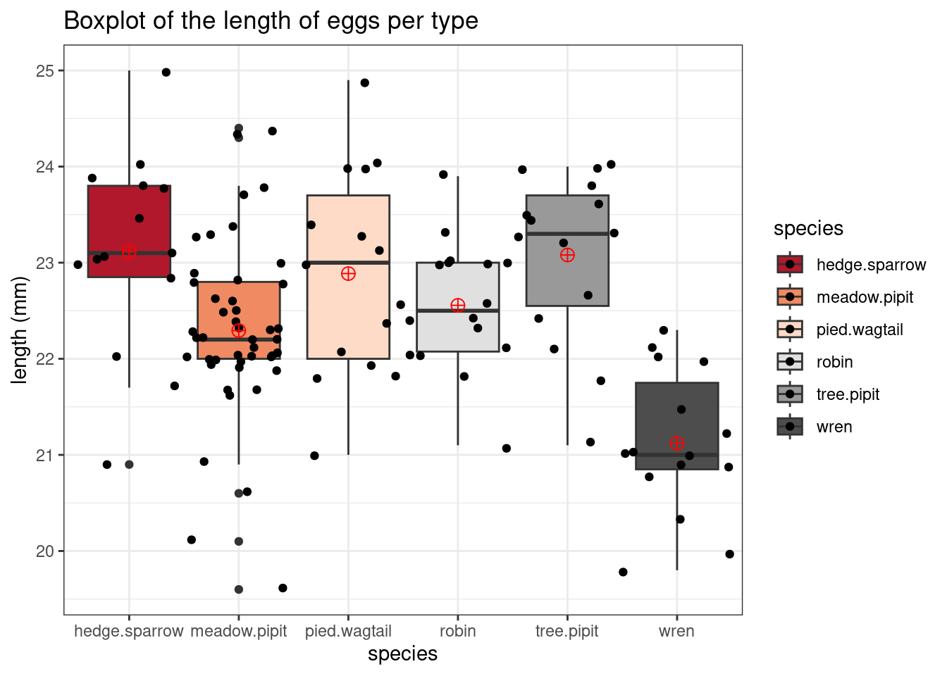
(1a) The boxplot of the length of the eggs across all the species is shown below. Based on these boxplots, do the assumptions of normality and similar variability appear to be met?
(1b) Formally verify that the assumptions are valid by using the outputs given.
Click for answer
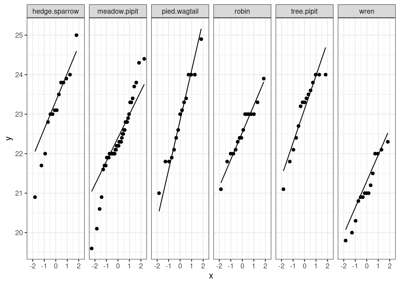
Answer: Based on the qqplot, the data points in each group are close to the line and there are no major deviations towards the center. So, the normality assumption seems to be satisfied.
Cuckoo %>%
ggplot(aes(sample=length)) + geom_qq() + geom_qq_line() + facet_grid(~species) + theme_bw() 
Similarly, based on the statistics below, the ratio of the largest \(s\) to the smallest \(s\) is \(1.57\). So, the equal variance assumption is satisfied.
Caution: If the equal variance assumption or the normality assumption is not met in ANOVA, then the results of the one-way ANOVA may not be reliable. This is especially true if the sample sizes between the groups are unequal and the variances between the groups are also unequal.
1.0722917/0.6821229[1] 1.571992library(dplyr)
stat <- Cuckoo %>% group_by(species) %>% summarize(mean(length), sd(length), length(length))
stat <- as.data.frame(stat)
stat species mean(length) sd(length) length(length)
1 hedge.sparrow 23.11429 1.0494373 14
2 meadow.pipit 22.29333 0.9195849 45
3 pied.wagtail 22.88667 1.0722917 15
4 robin 22.55625 0.6821229 16
5 tree.pipit 23.08000 0.8800974 15
6 wren 21.12000 0.7542262 15(1c) Fit an ANOVA model to do a formal hypothesis test. Report the test statistics and conclude your hypothesis test.
fit_anova <- aov(length~species, Cuckoo)
summary(fit_anova)
Df Sum Sq Mean Sq F value Pr(>F)
species 5 42.81 8.562 10.45 2.85e-08 ***
Residuals 114 93.41 0.819
---
Signif. codes: 0 '***' 0.001 '**' 0.01 '*' 0.05 '.' 0.1 ' ' 1
Click for answer
Answer: The hypotheses can be stated as:
\[H_0:\mu_1 = \mu_2 = \cdots = \mu_k\] \[H_a: \text{at least one } \mu_i \text{ is different}\]
Let’s assume the conditions for the test are approximately met. To find which of the species differ from the rest, we need to construct confidence intervals for the mean length differences between each pair of species.(1d) First, find a 95% confidence interval for the mean cuckoo egg length in European robin nests (Type = 4).
Click for answer
Answer:
95 \(\%\) confidence interval is:
MSE <- 0.8193847
stat[4,2] + c(-1,1)*(qt(1-0.05/2, df=113))*sqrt(MSE)/sqrt(stat[4,4])
[1] 22.10791 23.00459\[22.556 \pm 1.981*\frac{\sqrt{0.8194}}{\sqrt{16}}\] \[= (22.108, 23.005)\]
(1e) Find a 95% CI for the difference in mean egg length between European robin(type = 4) and Eurasian wren(type = 6) nests.
Click for answer
Answer:
(stat[4,2] - stat[6,2]) + c(-1,1)* (qt(1-0.05/2, df=113))* sqrt(MSE*(1/stat[4,4] + 1/stat[6,4]))[1] 0.79172 2.08078\[(22.556 - 21.120) \pm 1.981 \cdot \sqrt{0.8194\left(\frac{1}{16} + \frac{1}{15} \right)}\]
\(=(0.792, 2.081)\)
(1f) Find a 95% CI for the difference in mean egg length between Pied Wagtail (type = 3) and European robin(type = 4) nests.
Click for answer
Answer:
(stat[3,2] - stat[4,2]) + c(-1,1)* (qt(1-0.05/2, df=113))*sqrt(MSE*(1/stat[3,4] + 1/stat[4,4]))[1] -0.3141134 0.9749467(1g) We can use the R function pairwise.t.test to analyze which pair of means are significantly different from one another. Using p.adjust.method = "bonferroni", we will see the p-values adjusted for multiple comparison. These adjusted p-values should still be compared with \(\alpha = 0.05\) to find any significant differences.
Based on the R output, which of the pairs are different?
pairwise.t.test(Cuckoo$length, Cuckoo$species, p.adjust.method = "bonferroni")
    Pairwise comparisons using t tests with pooled SD

data:  Cuckoo$length and Cuckoo$species

             hedge.sparrow meadow.pipit pied.wagtail robin   tree.pipit
meadow.pipit 0.05554       -            -            -       -
pied.wagtail 1.00000       0.44898      -            -       -
robin        1.00000       1.00000      1.00000      -       -
tree.pipit   1.00000       0.06426      1.00000      1.00000 -
wren         5e-07         0.00045      7e-06        0.00035 5e-07

P value adjustment method: bonferroni
Click for answer
Answer:
Based on the adjusted p-values we can say the five pairs of species 6-1, 6-2, 6-3, 6-4, and 6-5 are different at the significance level of 5%. Here, each pairwise test is testing:
Problem 2: Metal Contamination
An environmental studies student working on an independent research project was investigating metal contamination in a local river. The metals can accumulate in organisms that live in the river (known as bioaccumulation). He collected samples of Quagga mussels at three sites in the river and measured the concentration of copper (in micrograms per gram, or mcg/g) in the mussels. His data are summarized in the provided table and plot. He wants to know if there are any significant differences in mean copper concentration among the three sites.
| Site | Mean (\(\bar{x}\)) | SD (\(s\)) | \(n\) |
|---|---|---|---|
| 1 | 21.34 | 3.092 | 5 |
| 2 | 16.60 | 2.687 | 4 |
| 3 | 13.16 | 4.274 | 5 |
(a) Assumptions
What do we need to assumption about copper concentrations to use one-way ANOVA to compare means at the three sites?
Click for answer
Answer: With such small sample sizes in each group it would be hard to get a good sense of how they are distributed. We will just need to assume that these measurements are approximately normally distributed.
(b) One-way ANOVA hypotheses
State the hypotheses for this test.
Click for answer
Answer: Let \(\mu_i\) be the true mean copper concentration at location \(i\). Then
\[ H_0: \mu_{1} = \mu_{2} = \mu_{3} \]
vs. \(H_A:\) at least one mean is different.(c) ANOVA table
Fill in the missing values A - E from the ANOVA table:
| Source | df | SS | MS | F |
|---|---|---|---|---|
| Groups | A = 2 |
169.05 | C = 84.525 |
E = 6.99 |
| Error | 11 | B = 132.97 |
D = 12.088 |
|
| Total | 13 | 302.02 |
Click for answer
Answer:
A: The group degrees of freedom is always the number of groups minus 1. Here we have 3 groups so \(A = 3-1=2\).
B: The group and error sum of squares adds up to the total sum of squares. So we have \(B = 302.02 - 169.05 = 132.97\).
C: Mean square values are always sum of squares divided by degrees of freedom. For groups MS: \(C = 169.05/2 = 84.525\)
D: Mean square values are always sum of squares divided by degrees of freedom. For error MS: \(D = 132.97/11 = 12.088\)
The F test stat is the ratio of the group MS and error MS: \(F = 84.525/12.088 = 6.992\).
302.02 - 169.05[1] 132.97169.05/2[1] 84.525132.97/11[1] 12.0881884.525/12.088[1] 6.992472(d) p-value
The command pf(x, df1=, df2=) gives the area under the F-distribution below the value x. Use this command to get the p-value from this one-way ANOVA test. Interpret this value.
Click for answer
Answer: The p-value is about 1.1%. If the means are the same at the three sites, we would see sample means this different, or even more different, about 1.1% of the time.
1-pf(6.992, df1=2, df2=11)[1] 0.01097789(e) Conclusion
What is your conclusion for this test?
Click for answer
Answer: We have some evidence that at least one of the true mean copper concentration at the three sites is differenct from the others.
(f) Confidence interval
Compute a 95% confidence interval for the difference in means between site 1 and 3. Interpret this interval.
Click for answer
Answer: Since we don’t have the data, we will have to compute the CI by hand. The degrees of freedom “best guess” (since we aren’t letting R approximate it), is \(11\). The 95% CI for the difference in true means in site 1 and 3 is :
\[ (21.34 - 13.16) \pm (2.201)) \sqrt{12.088\left(\dfrac{1}{5} + \dfrac{1}{5}\right)} = 3.34, 13.02 \]
(21.34 - 13.16) + c(-1,1)* qt(1-0.05/2, df = 11)*sqrt(12.088*(1/5+1/5))[1] 3.340234 13.019766We are 95% confident that the true mean copper concentration at site 1 is 3.34 to 13.02 mcg/g higher than the true mean concentration at site 3.