# load necessary libraries
library(readr) # read_csv
library(dplyr) # data manipulation
library(forcats) # categorical variables
library(janitor) # clean_names
library(tidyr) # drop_na
library(ggplot2) # for nice looking plotsPractice Problems 26
Linear Regression Analysis: Exploring the Relationship between Average Mathematics GPA and Length of Study in Mathematics
This class activity aims to guide you through a data analysis project involving a school score dataset. You will learn how to load a dataset, inspect its contents, manipulate and clean the data, perform exploratory analysis, and apply linear regression to identify relationships. Towards the end, you will deal with outliers and visualize data to comprehend the results better.
Step 1: Load and Inspect the Data
# Task: Load the school_scores.csv data file from your local directory
school_scores <- read_csv("data/school_scores.csv")
# Task: Use the glimpse() function to view the structure of your data.
# glimpse(school_scores)Step 2: Data Cleaning
# Task: Use janitor's clean_names() function to standardize column names,
# and tidyr's drop_na() to remove missing values.
school_scores_clean <- school_scores %>%
  janitor::clean_names() %>% # cleans column names
  tidyr::drop_na()  # removes all instances/rows where at least one NA exists
Step 3: Data Manipulation
# Task: Select relevant variables from the dataset for further analysis.
school_new <- school_scores_clean %>% select(year,
                                             state_name,
                                             total_math,
                                             total_verbal,
                                             academic_subjects_mathematics_average_gpa,
                                             academic_subjects_mathematics_average_years)
# Task: Create a new categorical variable named 'GPA' from
# the 'academic_subjects_mathematics_average_gpa' variable.
school_final <- school_new %>%
mutate(GPA_category = cut(academic_subjects_mathematics_average_gpa,
breaks = c(-Inf, 3, 3.25, 3.5, Inf),
labels = c("Low", "Satisfactory", "Good", "Excellent")))# Task: Collapse the GPA variable levels into two broad categories.
school_final <- school_final %>%
mutate(GPA_two_category = forcats::fct_collapse(GPA_category,
Low = c("Low", "Satisfactory"),
High = c("Good", "Excellent")))Step 4: Data Analysis - Linear Regression
# Fit a linear model
ggplot(data = school_final, aes(x = academic_subjects_mathematics_average_years,
                                y = academic_subjects_mathematics_average_gpa)) +
  geom_point() +
  geom_smooth(method = "lm", se = FALSE, color = "red", linetype = "dashed") +
  labs(x = "Average Years Studying Mathematics", y = "Average Mathematics GPA",
       title = "Linear Regression of Average Mathematics GPA vs. Length of Study") +
  theme_minimal()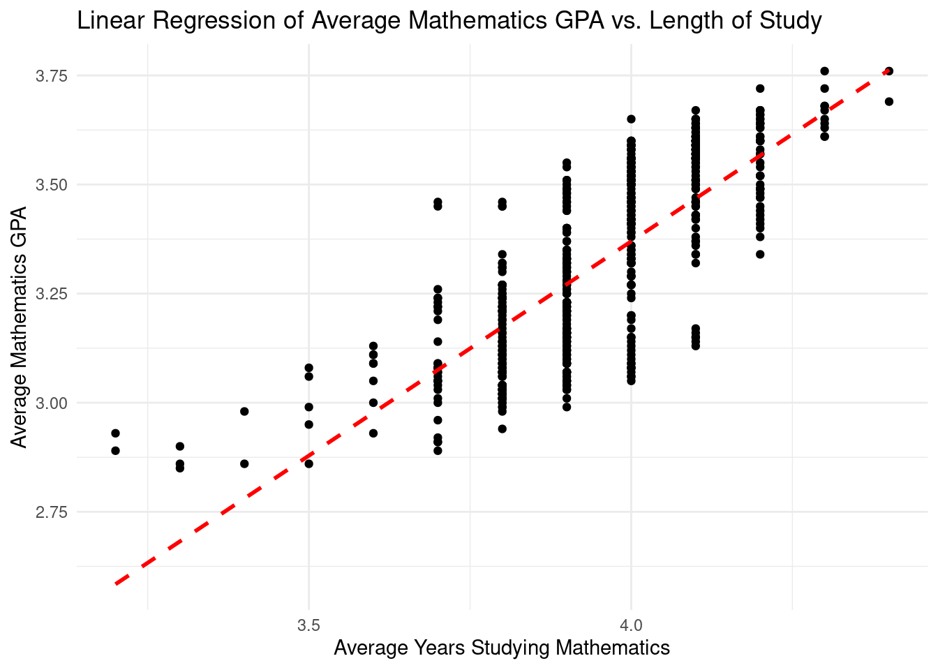
# Task: Conduct a linear regression analysis with GPA as the response
# variable and average years studying mathematics as the predictor.
GPA.lm <- lm(academic_subjects_mathematics_average_gpa ~
               academic_subjects_mathematics_average_years,
             data = school_final)
summary(GPA.lm)
Call:
lm(formula = academic_subjects_mathematics_average_gpa ~ academic_subjects_mathematics_average_years,
    data = school_final)

Residuals:
     Min       1Q   Median       3Q      Max
-0.33812 -0.10344  0.00478  0.11188  0.38478

Coefficients:
                                            Estimate Std. Error t value
(Intercept)                                  -0.5592     0.1348  -4.147
academic_subjects_mathematics_average_years   0.9823     0.0342  28.725
                                            Pr(>|t|)
(Intercept)                                 3.87e-05 ***
academic_subjects_mathematics_average_years  < 2e-16 ***
---
Signif. codes:  0 '***' 0.001 '**' 0.01 '*' 0.05 '.' 0.1 ' ' 1

Residual standard error: 0.138 on 575 degrees of freedom
Multiple R-squared:  0.5893,    Adjusted R-squared:  0.5886
F-statistic: 825.1 on 1 and 575 DF,  p-value: < 2.2e-16
# Task: Generate a Residual plot to assess the regression model's assumptions.
plot(GPA.lm, which = 1)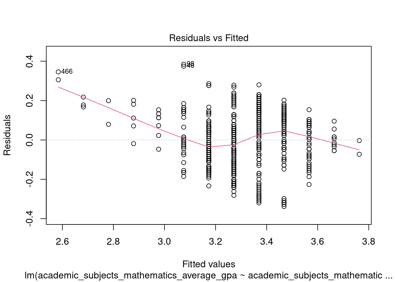
# Task: Generate a QQ plot to visualize the normality of residuals.
plot(GPA.lm, which = 2)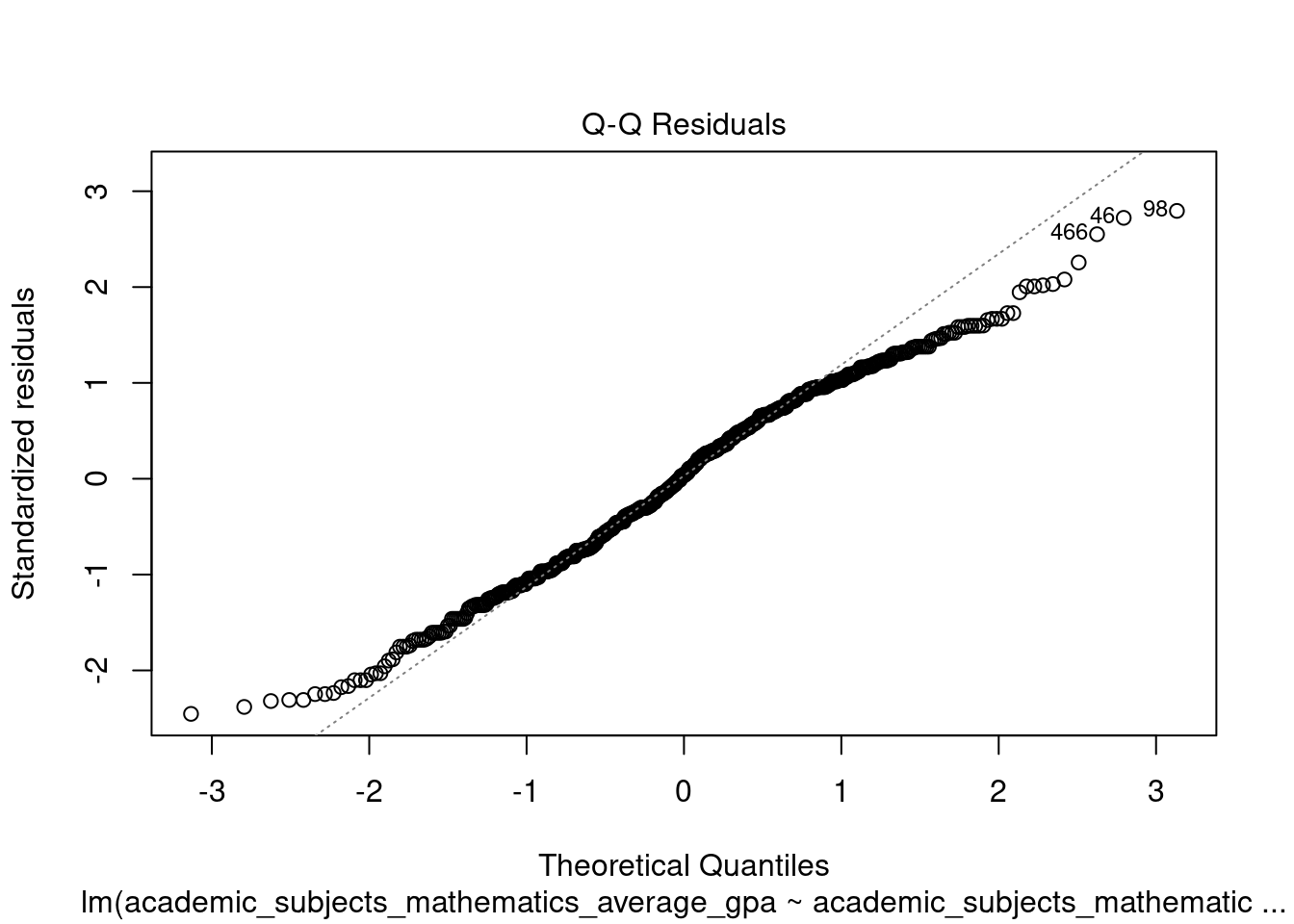
Step 5: Exploring the Relationship between Average Mathematics GPA and Length of Study
We will learn how to perform a t-test for the regression slope to identify if the average years studying mathematics significantly predict GPA in mathematics.
Hypothesis for Slope t-Test
The hypotheses for testing if the slope (\(\beta_1\)) of the regression line is significantly different from zero are:
- \(H_0: \beta_1 = 0\) (The slope is equal to zero - no relationship between the average years studying mathematics and GPA in mathematics.)
- \(H_1: \beta_1 \neq 0\) (The slope is not equal to zero - a relationship exists between the average years studying mathematics and GPA in mathematics.)
Conditions for Running t-Tests
The conditions for running a t-test on the slope of a regression line include:
- Linearity: The relationship between the predictor and response variable must be linear.
- Independence: The observations must be independent of each other.
- Normality: The residuals of the model should be approximately normally distributed.
- Equal Variance: The variance of residuals should be constant across the range of predictor variables.
Test Statistic
The test statistic for a slope t-test is calculated as:
\[ t = \frac{\hat{\beta}_1 - 0}{SE(\hat{\beta}_1)} \]
where \(\hat{\beta}_1\) is the estimated slope of the regression line, and \(SE(\hat{\beta}_1)\) is the standard error of the slope estimate.
Conducting the Slope t-Test
# Extracting the slope (Estimate) and its standard error
slope_estimate <- coef(GPA.lm)["academic_subjects_mathematics_average_years"]
slope_std_error <- summary(GPA.lm)$coefficients["academic_subjects_mathematics_average_years",
                                                "Std. Error"]

# Calculating the t-value
t_value <- slope_estimate / slope_std_error
t_value
academic_subjects_mathematics_average_years
28.72521 # Calculating the p-value
p_value <- 2 * pt(-abs(t_value), df = summary(GPA.lm)$df[2])
p_valueacademic_subjects_mathematics_average_years
3.285648e-113 Step 6: Handling Outliers
# Task: Filter the data to only include certain states.
school_selected <- school_final %>%
  filter(state_name %in% c("Alabama", "California", "Montana", "Minnesota", "Nevada"))
# Task: Visualize math SAT scores across GPA categories for the selected
# states using a boxplot, and identify potential outliers.
school_selected %>%
ggplot(aes(x=GPA_category,y=total_math,fill=GPA_category)) +
theme_bw() +
geom_boxplot() +
geom_jitter(width = 0.2) +
labs(title ="Boxplot of math SAT accross GPA categories",
y = "Average Math Score",
x = "GPA") +
stat_summary(fun=mean, geom="point", shape=10,
size=2, color="red", fill="black") +
ggthemes::theme_tufte()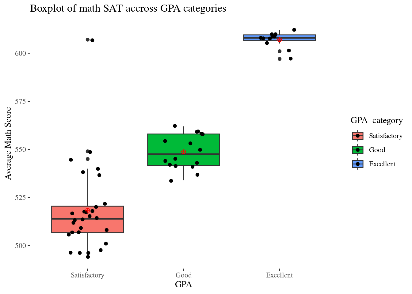
# Task: Remove outliers based on pre-determined conditions.
school_selected_no_outlier <-  school_selected %>%
  filter(GPA_category == "Excellent" & total_math >= 600 &  total_math <= 800 |
           GPA_category == "Good" & total_math >= 525  &  total_math <= 600 |
           GPA_category == "Satisfactory" & total_math >= 425  &  total_math <= 525)
Step 7: Visualizing Cleaned Data
# Task: Re-visualize the boxplot of math SAT scores across
# GPA categories after removing the outliers.
school_selected_no_outlier %>%
  ggplot(aes(x=GPA_category,y=total_math,fill=GPA_category)) +
  theme_bw() +
  geom_boxplot() +
  geom_jitter(width = 0.2) +
  labs(title ="Boxplot of math SAT accross GPA categories",
       y = "Average Math Score",
       x = "GPA") +
  stat_summary(fun=mean, geom="point", shape=10,
               size=2, color="red", fill="black") +
  ggthemes::theme_tufte()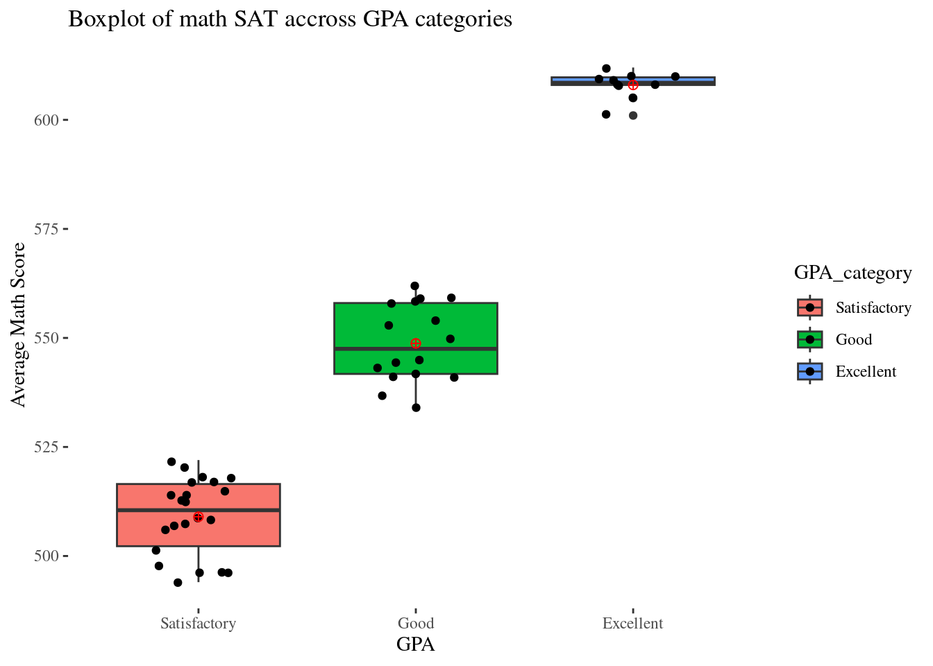
By the end of this activity, you will have practiced various data analysis techniques, including data manipulation, data cleaning, linear regression, slope t-test, and outlier handling, ultimately helping you understand the impact of GPA and length of study on student performance.